12. Map, Help and output files (🗺 Map, ⓘ Help)
Tabs: 🗺 Map, ⓘ Help · Code: tabs/tab_map.py, occurrence_map.py, study_area_figure.py, map_widget.py (figure options), tabs/tab_help.py, run_config.py, main_dialog.py (session log), main.py (crash log)
12.1 What this chapter covers
This chapter covers the two tabs that stand outside the workflow and the topics common to the whole workflow:
- The
🗺 Maptab: display of the inputs on an online basemap and a study area figure for publication (§12.3). - The
ⓘ Helptab: the built-in English guide and the update check (§12.4). - The complete file catalogue of the output folder (§12.5), the run record
habitus_run_config.json(§12.6), the session and crash logs (§12.7), environment variables (§12.8), troubleshooting (§12.9) and system requirements (§12.10).
Neither tab is locked; they can be used from the moment the program opens (main_dialog.py:194-196). They come after the numbered steps in the tab bar and provide no input to the workflow.
12.2 The place of the 🗺 Map tab
🗺 Map shows on a map what was given to ① Data before any model is built: the presence records, the records excluded before modelling once ① Data has been run, the user's own absence records, the study boundary and the calibration polygon. Its purpose is to see a misplaced record, swapped coordinates or a boundary layer that does not overlap the region before modelling (tabs/tab_map.py:1-11).
Each time the tab becomes visible, it rebuilds the map if the inputs have changed (tabs/tab_map.py:141-169). Model results are not shown here; the current and future maps are in the map viewer of the ③, ⑤ and ⑥ tabs (Chapters 6, 8, 9).
12.3 The 🗺 Map tab
At the top of the screen are the layer checkboxes and two buttons, below them a status line, and below that the map (tabs/tab_map.py:100-139). The map is drawn inside a web view with the Leaflet library; Leaflet ships with the program, while the basemap tiles are downloaded from tile.openstreetmap.org (occurrence_map.py:45-50, 92-95).
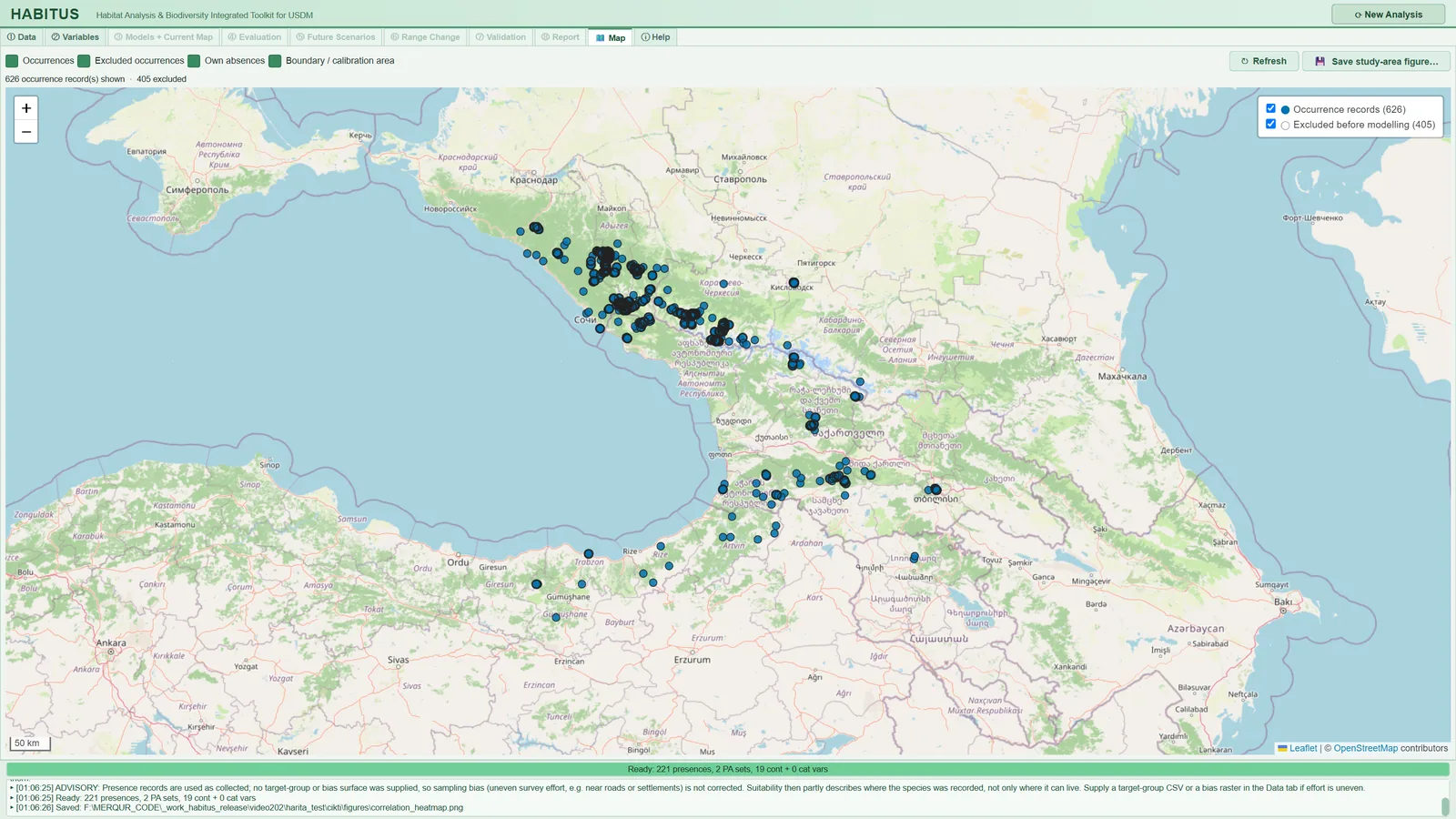
| Name in the UI | What it does | Default | Range / options | Code |
|---|---|---|---|---|
Occurrences |
Shows the presence records in the CSV; in a multi-species file each ticked species in a separate colour | on | on / off | tabs/tab_map.py:108, 179-214 |
Excluded occurrences |
Shows, with their reasons, the records excluded before modelling once ① Data has been run |
on | on / off | tabs/tab_map.py:109-113, 216-225 |
Own absences |
Shows the absence CSV given in the Own Absences sub-tab as black points |
on | on / off | tabs/tab_map.py:114, 227-243 |
Boundary / calibration area |
Draws the study boundary (red) and the calibration polygon (purple, dashed) | on | on / off | tabs/tab_map.py:115, 245-263 |
↻ Refresh |
Rebuilds the map from the inputs | — | button | tabs/tab_map.py:120-122 |
💾 Save study-area figure… |
Saves a location map for publication from the ticked layers | — | button; §12.3.2 | tabs/tab_map.py:123-130, 268-311 |
When one of the checkboxes changes, the map is redrawn immediately (tabs/tab_map.py:116-117). These checkboxes affect only the display and the saved figure; they do not change the data entering the modelling.
12.3.1 Contents of the layers
- Presence records. The columns are read with the names detected by
① Data, or, if none were detected, as the first three columns. In a single-species file the layer name is "Occurrence records"; in a multi-species file only the species ticked in① Dataare shown. Colours are taken from a colour-blind-safe list. The popup of each point gives the species name and the coordinates (tabs/tab_map.py:179-214,occurrence_map.py:40-42). - Excluded records. This layer is empty until
① Datahas been run. Reasons: "duplicate coordinate", "same raster cell as another record" (whenKeep one record per raster cellis on), "outside raster extent", "falls on NoData cell", "missing coordinate", "spatially thinned" and, for the absence file, "absence record outside extent or on NoData" (sdm_core.py:1853,1875,1899,1935,2779,2949,2966). In the sample run, 405 of the 626 records were excluded because another record was in the same cell (Figure 12.1). - Coordinate transformation. If the rasters are in a projected coordinate system, the records are transformed to longitude-latitude for display on the map; a single record that cannot be transformed is dropped and the others are unaffected (
tabs/tab_map.py:35-71). Before① Datahas been run, the coordinate system of the rasters is unknown; in that case, for coordinates in metres, the status line gives the warning "coordinates are not longitude/latitude in degrees and the rasters' CRS is not known yet: run ① Data first to place them correctly" (tabs/tab_map.py:196-199). - Decimation. If a layer has more than 20,000 points, every k-th point is drawn, for display only; the number in the layer list is the number of points drawn (
tabs/tab_map.py:22-24,313-326). - Polygons. The study boundary may be a polygon layer or a rectangle given by corner coordinates. The calibration polygon is drawn only when
Accessible areapolygonis selected. A geometry with more than 5000 vertices is simplified for display (tabs/tab_map.py:74-95,245-263).
The status line reports the number of records shown and excluded, the records without valid coordinates and the layers that could not be drawn. For a CSV that cannot be read, the message "The map could not be built: …" appears instead of the map (tabs/tab_map.py:154-169).
Note: The basemap tiles require a network connection. Without a connection the points and polygons are still drawn and the basemap remains blank. The program identifies itself to the OpenStreetMap tile server as "HABITUS/<version>" (
occurrence_map.py:7-11,53-58). If the web view component (PyQt6-WebEngine) is not installed, the tab shows the message "The map needs PyQt6-WebEngine, which is not installed (pip install PyQt6-WebEngine)." (occurrence_map.py:138-145).
12.3.2 Save study-area figure… (study area figure)
This button draws the ticked layers of the map, independently of the web view, as a location map that can be placed in a paper (study_area_figure.py:1-10). The OpenStreetMap tiles on screen are at screen resolution and carry their own licence terms; the saved figure instead uses the Natural Earth country boundaries (public domain) shipped with the program and needs no network.
Pressing the button first opens the "Figure for publication" options window, then the save dialog (tabs/tab_map.py:268-311).
| Name in the UI | What it does | Default | Range / options | Code |
|---|---|---|---|---|
Width: |
Width of the figure (journal column widths) | Double column — 174 mm |
Single column — 85 mm, 1.5 column — 120 mm, Double column — 174 mm |
map_widget.py:112-116, 193-196; tabs/tab_map.py:139 |
Resolution: |
Resolution for raster formats (PNG, TIFF, JPEG) | 600 dpi |
300, 600, 1200 dpi; not used for PDF, SVG, EPS | map_widget.py:117, 197-203 |
Title: |
Title text | names of the ticked species, otherwise the species name | free text | tabs/tab_map.py:283-288, map_widget.py:209-212 |
Include the title above the map |
Writes the title above the map | off | on / off | tabs/tab_map.py:139, map_widget.py:204-206 |
Italic title (scientific name) |
Writes the title in italics | on if there is a species name | on / off | tabs/tab_map.py:289 |
Locator map in the upper-left corner |
Adds a small locator map showing the study extent in the upper-left corner | on | on / off | tabs/tab_map.py:290, study_area_figure.py:265-290 |
| File type in the save dialog | The format is determined from the file extension | PNG | PNG, TIFF (LZW-compressed), PDF, SVG, EPS (vector), JPEG (quality 95) | map_widget.py:156-177 |
The suggested file name is <species>_study_area.png in the output folder (tabs/tab_map.py:294-300). The window remembers the last choices during the session (tabs/tab_map.py:293).
The figure consists of the following elements (study_area_figure.py:190-262, 293-313):
- Extent. An 8% margin around everything drawn; if the width or height is less than 0.5 degrees, it is widened to 0.5 degrees.
- Background. Natural Earth countries; boundaries at 1:10 million scale if the long side of the extent is less than 20 degrees, otherwise at 1:50 million. Sea is light blue, land light grey.
- Layers. Boundary and calibration polygons, presence records, excluded records (hollow) and own absences; in the legend the name of each layer and "(n = <number of records>)".
- Map elements. Axes labelled in degrees, dashed graticule, scale bar, north arrow; aspect-ratio correction by the cosine of the mid-latitude.
- Locator map. An area 6 times the study extent (3 times if the extent exceeds 30 degrees); the extent is shown with a red frame.
- 180° meridian. If the data lie on both sides of the 180th meridian and are closer to each other across that line, 360° is added to western longitudes; the region is drawn in one piece.
-
Text. Arial (otherwise Helvetica, Liberation Sans, DejaVu Sans) 7-9 pt, white background; in PDF, SVG and EPS the font is embedded (
map_widget.py:149-153,219). -
What it does. Produces the "study area" figure of a paper without leaving the program, at column width and true resolution.
- When and how to set it. If the journal wants a single-column figure, choose 85 mm; for a full page, 174 mm. Because the map contains fine text and lines, 600 dpi is sufficient for most journals; if a vector format (PDF, EPS) is required, the resolution is not used. Because most journals want the title in the figure caption,
Include the title above the mapis off by default. - Effect on results. It does not affect the model result. The figure draws the layers ticked in the Map tab; if a layer's checkbox is off, it is absent from the figure too.
- Caution. If there is nothing to draw, the message "Nothing to draw yet: load records or a study boundary in ① Data." appears. If the coordinates are not in degrees, the figure is refused with the message "The coordinates are not longitude/latitude in degrees … Run (1) Data first so that projected coordinates are converted, or check that longitude and latitude are not swapped." (
study_area_figure.py:64-69,tabs/tab_map.py:278-282). For decimated layers (more than 20,000 points) the figure also draws the decimated points. Files whose names end in_study_area.pngare not taken into the map section of⑧ Report(tabs/tab_report.py:1802-1803).
12.4 The ⓘ Help tab
ⓘ Help is a user guide embedded in the program, in English only (tabs/tab_help.py:1000-1017). The top bar holds the update buttons, with twelve page tabs below it (tabs/tab_help.py:1027-1101).
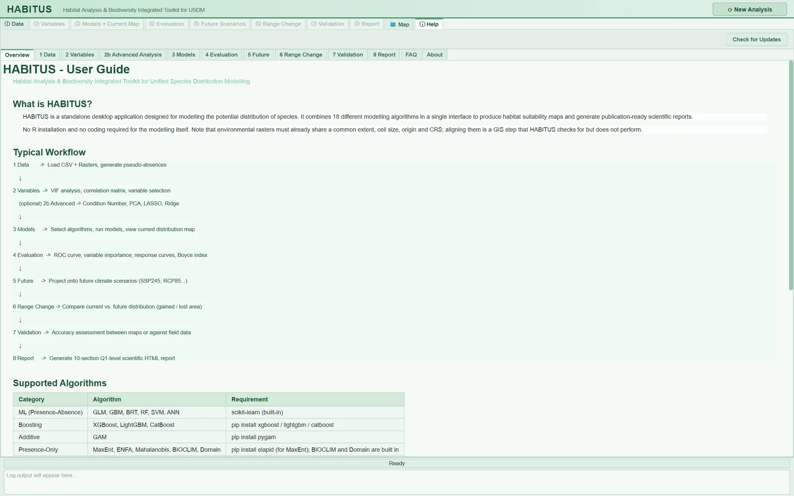
| Page | Contents |
|---|---|
Overview |
Description of the program, the eight-step workflow, the algorithm table and the required libraries, quick start |
1 Data |
Presence CSV, rasters, background and pseudo-absence settings, output folder |
2 Variables |
VIF and correlation, colour codes, confirmation |
2b Advanced Analysis |
Condition number, PCA, LASSO, Ridge and how to read them together |
3 Models |
Algorithm selection, minimum-record recommendations, training settings, rationale of the cross-validation design, two-level ensemble, performance metrics, current map |
4 Evaluation |
Sub-tabs, ROC, variable importance, response curves, threshold methods |
5 Future |
Scenario name, algorithm selection, adding future rasters |
6 Range Change |
Result codes (-2, 0, 1, 2), file selection, reading the result table |
7 Validation |
Map selection, reclassification, sampling, metrics, export, interpreting Kappa |
8 Report |
Report sections, generation and export, ODMAP protocol, map quality |
FAQ |
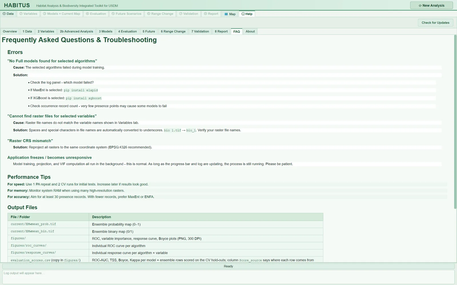
Common errors, performance tips, output files table |
About |
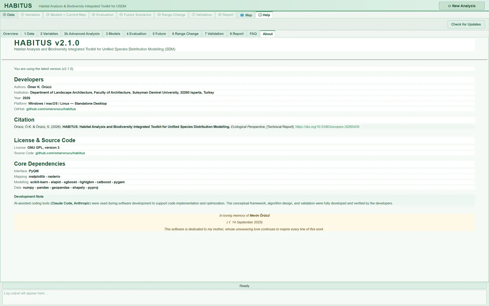
Version, developer, citation, licence (GNU GPL version 3), core dependencies, update status |
| Name in the UI | What it does | Default | Range / options | Code |
|---|---|---|---|---|
Check for Updates |
Manually asks whether there is a new version on the release page; the result appears on the About page |
— | button | tabs/tab_help.py:1052-1059, 1142-1152 |
Download Update |
Appears when a new version is found; downloads the installer for this computer to the Downloads folder | hidden | button | tabs/tab_help.py:1062-1071, 1154-1248 |
The program performs the update check automatically, in the background, at start-up; it does not do so if the environment variable HABITUS_NO_UPDATE_CHECK is defined (main_dialog.py:130-143). The query goes to the GitHub release page and is abandoned if no response arrives within 10 seconds (updater.py:88-94). The About page shows the result of the check in a banner: "Checking for updates...", "You are using the latest version (v…)", "Update Available - v…" or "Update check failed: …" (tabs/tab_help.py:1103-1140). If a new version is found, a line is also written to the log panel (main_dialog.py:145-148).
Download Update downloads the installer but does not install it: "Close HABITUS and run it to install the update. Your settings and results are not touched." (tabs/tab_help.py:1212-1218). If the download fails, the address of the release page is given.
Note: The Help pages are a short reference guide. For exact details (default values, file names) this book should be taken as authoritative; for example, the actual names of the output files are in §12.5.
12.5 File catalogue of the output folder
All outputs go to the ① Data > Output Directory folder (or to the folder entered in ③ Models) (Section 1.9). In a multi-species file each species is in its own subfolder; that subfolder carries the same tree as below, while the parent folder holds batch_summary.csv and (if there is a boundary) masked_inputs/current/.
The <species> prefix in file names: in projection, report and figure files, spaces in the species name are converted to underscores (abies_nordmanniana_current_EMwmean_prob.tif); in the range change file the species name stays as it is (abies nordmanniana_SSP585_2090_SRC.tif) (sdm_core.py:7655-7656, tabs/tab_range.py:213-216). If the species name is unknown, no prefix is added.
The tree below is taken from the folder of the sample run and completed from the code:
<output folder>/
  habitus_run_config.json             ③ run record
  evaluation_scores.csv               ③ (+ evaluation_scores.<time>.bak.csv)
  .habitus_state.json                 summary for the CSV backup check
  occurrence_train.csv                ③ training presences
  occurrence_test.csv                 ③ test presences
  occurrence_all_splits.csv           ③ both together
  occurrences_used.csv                ① multi-species file only
  accessible_area.tif                 ① accessible area
  background_maxent.csv               ① optional
  <species>_<YYYYMMDD_HHMMSS>.log     session log
  <species>_HABITUS_report_<time>.html ⑧ report
  odmap_protocol.md / .csv            ⑧ via the ODMAP button
  <species>_<analysis name>_SRC.tif   ⑥ range change
  <species>_study_area.png            🗺 optional
  masked_inputs/current/              ① rasters clipped to the boundary
  masked_inputs/<scenario>/           ⑤ scenario rasters clipped to the boundary
  current/                            ③ current-climate maps
  <scenario>/                         ⑤ future maps
  figures/                            ② ④ figures and tables
  advanced_analysis/                  ② Advanced Analysis export
  tuning/tuning_<algorithm>.csv       ③ Tuning
  validation/                         ⑦ reclassified rasters
| File | Which step | Contents | Code |
|---|---|---|---|
accessible_area.tif |
① Data | Accessible area mask from which the background is drawn; not written if Accessible area is none. Used by ⑥ Range Change |
tabs/tab_data.py:1540-1545 |
background_maxent.csv |
① Data | MaxEnt background points and their environmental values (if requested in the MaxEnt sub-tab) | tabs/tab_data.py:1550-1559 |
occurrences_used.csv |
① Data | In a multi-species file, the records of this species only | tabs/tab_data.py:1503 |
masked_inputs/current/, masked_inputs/<scenario>/ |
① Data, ⑤ Future | Raster copies clipped to the study boundary | tabs/tab_data.py:1520, tabs/tab_projection.py:607 |
figures/correlation_heatmap.png, correlation_heatmap_selected.png, vif_barplot.png |
② Variables | Correlation heat map (all and selected variables), VIF plot | tabs/tab_vif.py:1007, 1151, 1278 |
figures/high_correlation_pairs.csv, figures/variable_priority_ranking.csv |
② Variables | Highly correlated pairs; VIF and priority ranking | tabs/tab_vif.py:1056, 1091 |
advanced_analysis/ |
② Advanced Analysis | pca_variance.png/.csv, pca_loadings.csv, lasso_coefficient_paths.png, lasso_coefficients.csv, lasso_path.csv, ridge_coefficient_paths.png, ridge_coefficients.csv, ridge_path.csv |
tabs/tab_vif_advanced.py:769-882 |
current/<species>_current_<ALGO>_PA<n>_prob.tif, _bin.tif |
③ Models | Probability (0-1) and binary (0/1) map for each algorithm and pseudo-absence set | sdm_core.py:7895, 7911 |
current/<species>_current_<ALGO>_mean_prob.tif, _mean_bin.tif, _sd.tif |
③ Models | Mean and standard deviation of the within-algorithm replicates | sdm_core.py:7981-8005 |
current/<species>_current_EMwmean_prob.tif, EMca_prob.tif (and _bin) |
③ Models | Ensemble: weighted mean and committee averaging | sdm_core.py:8083, 8098 |
current/<species>_current_EMsd.tif |
③ Models | Spread among ensemble members (not thresholded) | sdm_core.py:8056-8066 |
current/<species>_current_NT1.tif, NT2.tif, MIC_NT1.tif, MIC_NT2.tif |
③ Models | Extrapolation diagnostic (ExDet) and most influential variable | sdm_core.py:7205-7215 |
current/<species>_current_projection_options.json |
③ Models | Projection options (clamp, MESS) and grid alignment summary | sdm_core.py:7655-7662 |
evaluation_scores.csv (a copy in figures/) |
③ Models, ④ Evaluation | ROC-AUC, TSS, Boyce, Kappa etc. for each model and ensemble; the Score_source column states the source of the score |
tabs/tab_evaluation.py:1073-1107 |
occurrence_train.csv, occurrence_test.csv, occurrence_all_splits.csv |
③ Models | Training and test points with the columns longitude, latitude, presence, split |
tabs/tab_models.py:1915-1955 |
habitus_run_config.json |
③ Models | Run record (§12.6) | tabs/tab_models.py:1640-1657 |
tuning/tuning_<algorithm>.csv |
③ Tuning | Grid search table | tabs/tab_tuning.py:408-413 |
figures/evaluation_model_scores.png, evaluation_roc_curves.png, evaluation_omission_pr_calibration.png/.csv, evaluation_variable_importance.png, evaluation_response_<ALGO>.png, evaluation_boyce_<ALGO>.png |
④ Evaluation | Evaluation figures (300 dpi) and the omission-calibration table | tabs/tab_evaluation.py:353-847, 923-937 |
figures/classification_thresholds.csv |
④ Evaluation | Thresholds found by each threshold method and hold-out performance | tabs/tab_evaluation.py:1323 |
<scenario>/<species>_<scenario>_…tif |
⑤ Future | The same family of files as current/, with the scenario name |
sdm_core.py:7895-8138 |
<species>_<analysis name>_SRC.tif |
⑥ Range Change | Change map: -2 loss, 0 stable absence, 1 stable presence, 2 gain | tabs/tab_range.py:213-216 |
validation/Reclassify_ref_<name>.tif, Reclassify_val_<name>.tif |
⑦ Validation | Reclassified reference and model maps | tabs/tab_validation.py:728-730, 819-830 |
validation_report_<time>.txt/.json/.html, validation_points_<time>.csv |
⑦ Validation | Validation report and sample points, if the user saves them | tabs/tab_validation.py:970-1005 |
<species>_HABITUS_report_<time>.html |
⑧ Report | Single-file HTML report; the figures are embedded in the file | tabs/tab_report.py:2507-2510 |
odmap_protocol.md, odmap_protocol.csv |
⑧ Report | Partially filled ODMAP protocol | odmap.py:647-686 |
batch_summary.csv |
⑧ Report (batch) | Per species: status, failed step, error, folder, duration | batch_species.py:280 |
<species>_<YYYYMMDD_HHMMSS>.log |
all steps | Session log (§12.7) | main_dialog.py:612-645 |
Raster format. Projection rasters are GeoTIFF, float32, NoData value -9999 (sdm_core.py:7205-7215). Probability maps are in the range 0-1. In the current/ folder of the sample run, 37 map files were written for four algorithms (Figure 1.3).
Caution: A new run overwrites the files in the output folder; files left from a previous run and not produced in the new run are not deleted (Section 1.6.2). If
evaluation_scores.csvhas been edited by hand, it is backed up as<name>.<YYYYmmdd_HHMMSS>.bak.csvbefore being overwritten; for this, a summary of the file's last write is kept in the.habitus_state.jsonfile (sdm_core.py:6752-6800).
12.6 Run record: habitus_run_config.json
The run record gathers the information needed to reconstruct an analysis in a single machine-readable file (run_config.py:1-14). Each time ③ Models runs, it is written to the root of the output folder after modelling has finished (tabs/tab_models.py:1640-1657, run_config.py:154-163).
12.6.1 Top-level fields
| Field | Contents | Sample run | Code |
|---|---|---|---|
habitus_version |
Program version | "2.1.0" | run_config.py:140 |
random_seed |
Seed of the run | 42 | run_config.py:141 |
started, finished |
Time the record was created and written (ISO format) | both "2026-11-21T05:11:12" | run_config.py:97-98, 142-143 |
settings |
Settings section by section (§12.6.2) | 9 sections | run_config.py:144 |
setting_source |
Source of each setting: default, user or recorded |
36 default, 2 user, 44 recorded |
run_config.py:79-92, 105-119 |
defaults_left_unchanged |
List of settings left at their defaults: {section, setting, value} |
36 items | run_config.py:127-134, 146-149 |
notes |
ADVISORY: notes and the cross-validation summary |
4 lines | run_config.py:121-125 |
environment |
Python version, operating system, processor architecture, versions of the scientific packages | Python 3.13.1, Windows 11, AMD64, numpy 2.4.6, scikit-learn 1.8.0, elapid 1.0.4 … | run_config.py:61-74 |
started and finished are not the start and end of the modelling job; they show the moment the record was created and written. The duration of the job is read from the time stamps in the session log.
Setting source. The code compares each recorded value with the program's default (run_config.py:105-119):
default: the value equals the program's default;user: the setting has a default and the user changed it;recorded: there is no default to compare with; it is either an input given by the user (presence file, rasters) or a quantity found during the run (number of presences used, block size, prevalence).
The defaults_left_unchanged list is also printed explicitly in the report; thus no default enters a publication without the user being aware of it (run_config.py:87-91).
12.6.2 settings sections
| Section | Main fields | Chapter |
|---|---|---|
data |
presence file, species, numbers of records used and excluded and the reasons, one record per cell, rasters, raster grid (shape, cell size, CRS), prevalence | 2 |
background |
absence source (pseudo, user, user+pseudo), strategy, numbers of replicates and points, MaxEnt background, sampling bias correction |
3 |
study_area |
accessible area method, buffer, percentage of the extent, calibration layer | 3 |
study_boundary |
boundary layer, number of polygons, clipped grid | 2 |
thinning |
whether thinning was applied, distance, records kept and dropped | 3 |
spatial_structure |
spatial autocorrelation range and method, study extent | 5 |
cross_validation |
design, requested number of folds, block size, the design actually used in each pseudo-absence set (per_pa_set) |
5 |
models |
algorithms and all their options, threshold method, Boyce formula, variables, clamp, categorical variables, class weight | 5-6 |
ensemble |
ensemble method, minimum score, weights, surfaces written, hold-out ensemble scores | 6 |
tuning_<algorithm> |
If Tuning was done, the grid, the rule and the selected point | 6 |
From the sample run: data.n_presences_used 143, data.n_points_dropped 483, data.prevalence 0.125; in notes, "Cross-validation: PA1: spatial_block, 4 fold(s), blocks of 151.5 km [SSB=0.36] | PA2: …".
Note: The file is written when
③ Modelsfinishes. The settings of later steps are not here: the projection options are in the<species>_<scenario>_projection_options.jsonfile in each scenario folder; the⑥ Range Changeand⑦ Validationsettings are in the session log and the report. The program's internal constants (e.g. fixed values other than the ranges of the Tuning grid) are not written to the record; the record contains the values collected from the UI and passed to the computation engine.
12.6.3 The run record and ODMAP
ODMAP (Overview, Data, Model, Assessment, Prediction) is the standard protocol proposed for reporting species distribution models (Zurell et al., 2020). The ODMAP button in ⑧ Report fills in the elements of the protocol by reading the run record (odmap.py:1-22, 155-200; Chapter 11):
- Elements that have a counterpart in the record (
auto) are filled in: record counts, predictors, cross-validation, algorithms, threshold, ensemble etc. - Elements the program cannot know (authors, hypotheses, data sources, model objective) are marked
user_requiredand carry the text "Not recorded by HABITUS: to be completed by the user." (odmap.py:38,153-154). - If the run record cannot be found, the protocol is still written, but every element becomes
user_required(tabs/tab_report.py:545-565).
In short, the run record is the source of the protocol; the ODMAP file is a readable, standard-format summary of the record. The protocol does not count as an "ODMAP-compliant report" until the user completes the missing elements.
12.7 Logs
12.7.1 Session log
From the moment the output folder is known, every line of the log panel is also written to the <species>_<YYYYMMDD_HHMMSS>.log file in the folder (Section 1.7; main_dialog.py:612-645, 790-801). The file contains:
- a header: "HABITUS Analysis Log", species, start time;
- each message in the form
[HH:MM:ss] message; every raster read, numbers of excluded records, the autocorrelation range, the duration of each model, every file saved, warnings andADVISORY:notes; - for errors, the full error text under the heading
--- ERROR ---; - at closing, a "Closed" line.
The log of the sample run (habitus_20261121_050108.log) begins as follows: "[05:01:08] Reading raster 1 of 19: bio_1.tif" … "[05:01:09] ⚠ 405 of 626 presence records removed (405 in a cell that already has a record) — 221 retained, one per raster cell." … "[05:01:09] Spatial autocorrelation range = 151.5 km (variogram)." ⑧ Report appends the log file in the output folder to the last section of the report (tabs/tab_report.py:607-616).
12.7.2 Crash log
If the program closes before it can show an error window (a native crash or an uncaught error), the cause is written to the crash log in the user data folder (main.py:253-290):
| Platform | Folder |
|---|---|
| Windows | %LOCALAPPDATA%\HABITUS\logs\ |
| macOS | ~/Library/Application Support/HABITUS/logs/ |
| Linux | $XDG_DATA_HOME/HABITUS/logs/, or ~/.local/share/HABITUS/logs/ if the variable is not set |
There is one file per day (crash_YYYYMMDD.log); each start-up adds a line with the version number and time. In a native crash, the Python stack of all threads at that moment is written. When reporting a crash, this file should be sent together with the session log.
12.8 Environment variables
Environment variables are defined in the operating system before the program is started. None of them is needed in ordinary use.
| Variable | Effect | Default | Code |
|---|---|---|---|
HABITUS_UI_SCALE |
Proportionally enlarges or shrinks the UI text and controls | 1.0; a value outside 0.5-3.0 or an invalid value is taken as 1.0 | ui_style.py:30-38 |
HABITUS_PROJECTION_TILE_CELLS |
Number of cells in a strip when projecting large rasters; 0 turns striping off. A raster smaller than twice this value is processed in one piece | 2000000 | sdm_core.py:7512-7526 |
HABITUS_NO_UPDATE_CHECK |
Any non-empty value turns off the update check at start-up (offline environment) | undefined | main_dialog.py:131-132 |
HABITUS_SAFE_GRAPHICS |
Linux launch scripts only: if 1, software rendering is enabled (if windows open blank) |
undefined | scripts/make_linux_archive.sh:71-75 |
QT_QPA_PLATFORM |
Linux scripts: in a Wayland session, xcb (XWayland) is selected if it is not defined; the user's value is kept |
set by the script | scripts/make_linux_archive.sh:63-66 |
QTWEBENGINE_DISABLE_SANDBOX |
Linux scripts set it to 1 so that the web view of the Map tab can run from the portable folder |
set by the script | scripts/make_linux_archive.sh:67-70 |
PROJ_DATA, PROJ_LIB |
If they do not point to a valid coordinate database, the program sets them to its own copy at start-up | checked by the program | main.py:110-163 |
PYTHONHASHSEED |
If not defined, set to the run seed when ① Data runs |
seed | run_config.py:49 |
HABITUS_OWNER_PID |
Internal use: the running program writes its own process number; helper processes derived from it do not open a second window. Should not be set by hand | written by the program | proc_guard.py:46, 86-122 |
12.8.1 HABITUS_PROJECTION_TILE_CELLS
- What it does. During projection the raster is divided into row strips; each strip is predicted separately and the files are merged (
sdm_core.py:7514-7526). - When and how to set it. If an out-of-memory error occurs, the value is reduced (e.g. 500000). If memory is plentiful and speed matters, it can be increased.
- Effect on results. According to the code comment, striped projection is designed to produce the same files as single-piece projection (
sdm_core.py:7531-7537); the strip size changes memory use and run time. Striped and single-piece outputs have not been compared separately for this book. - Caution. A non-numeric value falls back to the default (2000000) (
sdm_core.py:7521-7524).
12.9 Troubleshooting
The full error text is obtained with the Copy full message button in the error window and is found in the session log (Section 1.7). The messages below are taken from the code (their beginnings are given).
| Message | Cause | Solution | Code |
|---|---|---|---|
| "Please specify an output directory." | Output Directory is empty |
Select a folder, or first select a CSV and wait for the automatic folder | tabs/tab_data.py:1370-1371 |
| "Environmental rasters are not on the same grid." | One of the rasters differs from the first raster in size, cell size, origin or CRS; the message names the differing file | Bring the rasters to a common grid in a GIS program or give a study boundary (Chapter 2) | sdm_core.py:1735-1742 |
| "No continuous environmental rasters were given." | Only categorical rasters were added | Add at least one continuous raster | sdm_core.py:1554 |
| "Only N valid presence point(s) remain after removing …" | Most records are outside the raster or on NoData; usually the CSV and the rasters have different coordinate systems | Check the coordinate system and the longitude-latitude order; look at the records in 🗺 Map |
sdm_core.py:2028-2036 |
| "No presence record can be used: the layer(s) … have no value (NoData) …" | The named layer is NoData at all records | Check the layer or remove it | sdm_core.py:2021 |
| "N of M coordinate pair(s) are not valid degrees" | Coordinates in metres or columns reversed | Correct the CSV | sdm_inputs.py:192 |
| "Only one predictor is loaded …" | A single continuous raster | Add rasters in ① Data |
tabs/tab_vif.py:369 |
| "… is too small for N requested points: the background was drawn from the FULL raster extent instead." | The accessible area is too narrow for the requested number of points | Enlarge the buffer or reduce the number of points | sdm_core.py:2845 |
| "Calibration polygon: NONE of the N presence records lies inside the polygon(s)." | The polygon is in another region or another CRS | Check the polygon | sdm_core.py:2657 |
| "WARNING: … were merged into others …" | The block design could not provide the requested number of folds | Reduce the number of folds or the block size (Chapter 5) | sdm_core.py:5131 |
| "WARNING (design not applied): …" | The requested cross-validation design could not be applied and random folds were used instead; scores may be optimistic | Review the design and the distribution of records (Chapter 5) | sdm_core.py:5139 |
| "No model passed the ensemble threshold …" | No model passed the threshold for entering the ensemble | Lower the minimum score or choose another metric (Chapter 6) | tabs/tab_models.py:1732 |
| "No Full models found for selected algorithms." | The selected algorithms failed in training | Look at the FAILED lines in the log; check that the library is installed |
sdm_core.py:7859 |
| "Raster count mismatch! …" | The number of future rasters does not match the model's variables | Check the scenario folder and the file names (Chapter 8) | tabs/tab_projection.py:527 |
| "Cannot find raster files for N selected variable(s)" | Scenario file names do not match the variable names | Match the file names to the names in ② Variables |
tabs/tab_models.py:1435 |
| "Complete the workflow for one species first …" | For a batch run, ①-③ must first be completed for one species | Run one species to the end (Chapter 11) | tabs/tab_report.py:481 |
| "ODMAP protocol: No output folder yet. Run the models first." | No output folder | Run ③ Models first |
tabs/tab_report.py:554 |
| "… still running — close anyway?" | The window is being closed while a job is running | Yes cancels the job; wait for it to finish |
main_dialog.py:293-301 |
| "Unable to allocate …" / "MemoryError" | Insufficient memory | Clip the rasters, reduce the number of points, reduce HABITUS_PROJECTION_TILE_CELLS |
error_dialog.py:39-41 |
| "proj.db lacks DATABASE.LAYOUT.VERSION.MAJOR …" | Another installation of the coordinate library interferes | The program selects its own copy at start-up; if it persists, remove the PROJ_DATA and PROJ_LIB variables |
main.py:82-110 |
| "Permission denied" / "being used by another process" | The output file is open in another program | Close the file and run again | error_dialog.py:51-53 |
| "The map needs PyQt6-WebEngine, which is not installed" | The web component of the Map tab is missing (running from source) | pip install PyQt6-WebEngine |
occurrence_map.py:140-141 |
| Basemap blank in the Map tab | No network connection or the tile server does not respond | Check the connection; the points and Save study-area figure… work offline |
occurrence_map.py:92-95 |
| Windows open blank on Linux | Graphics driver problem | Start with HABITUS_SAFE_GRAPHICS=1 |
scripts/make_linux_archive.sh:71-75 |
| Program closed without a message | Native crash | Send the crash log (§12.7.2) | main.py:253-290 |
| Window seems unresponsive | A long job is running in the background | If the progress bar and the log are updating, wait | threads.py |
Tip: To test whether an installation is sound, first run
--selftest(Section 1.3). The report names missing algorithm libraries and coordinate database problems.
12.10 System requirements
| Item | Requirement | Source |
|---|---|---|
| Windows | 64-bit Windows 10 (version 1809, build 17763) or later; Windows 11 | habitus_setup.iss:33, 44 |
| macOS | Separate Apple Silicon and Intel packages; the minimum system version is stated on the package | habitus.spec:345-373 |
| Linux | 64-bit; distributions with glibc 2.35 or later (the packages take some system libraries, e.g. GL and X11, from the system) | CHANGELOG.md, Linux packages |
| Running from source | Python 3.10 or later and the requirements.txt dependencies |
pyproject.toml:11 |
| Memory | There is no lower limit in the code; the memory needed depends on the size and number of rasters. A measured example: 19 global layers (2.5 minutes) occupy about 2.6 GB in memory | CHANGELOG.md |
| Network | Not required. Only the basemap tiles of the Map tab and the update check connect to the network | occurrence_map.py:92, updater.py:88 |
| Screen | The window opens at up to 95% of the screen; on a small screen the tabs scroll. Text can be enlarged with HABITUS_UI_SCALE |
main_dialog.py:113-121, ui_style.py:30-38 |
The measure that reduces the memory requirement most is clipping the rasters to the study region with ① Data > Study Boundary (Chapter 2). The run times of the algorithms are written to the session log; before a large analysis, a small trial (one pseudo-absence replicate, few algorithms) helps to estimate the run time.
12.11 Expert questions
Q1. Can another researcher reconstruct this study from the output folder alone?
Answer: Largely. habitus_run_config.json carries the seed, the paths of the input files, all UI settings, the cross-validation design actually applied and the package versions (run_config.py:137-152; tabs/tab_models.py:2056-2242). The input files themselves are not copied into the folder (except the copies clipped with the study boundary, masked_inputs/); only their paths are written. No checksum proving that the content of the rasters has not changed is written to the record. The projection settings are in separate projection_options.json files. For full reconstruction the input data must be archived separately.
Q2. Why is defaults_left_unchanged a separate list?
Answer: To separate which numbers in a publication were chosen deliberately and which remained as the program's defaults. The code compares each setting with its default and puts those equal to the default into this list (run_config.py:105-134); the report prints this list. In the sample run 36 settings are at their defaults. A reviewer can use this list to ask, for example, whether the number of pseudo-absences (1000) or the number of folds was justified.
Q3. What does the recorded source mean, and how does it differ from user?
Answer: user is only for settings that have a default and that the user changed. Values without a default (input files, the block size computed during the run, prevalence, number of records used) are marked recorded (run_config.py:79-92, 113-118). Thus a computed number does not look like a user choice. In the sample run 44 values are recorded and 2 are user.
Q4. Does the run record replace an ODMAP report?
Answer: No. ODMAP (Zurell et al., 2020) includes elements the program cannot know, such as authorship, objective, hypotheses and data sources. odmap.py fills in the elements that have a counterpart in the record as auto, leaves the others as user_required and does not invent any value (odmap.py:14-22, 153-154). According to the code comment, the elements are those of Table 1 of the paper; the detailed question list in the supplementary table was not used as the basis (odmap.py:11-14). The user must complete the user_required rows.
Q5. Can the output maps be used directly in another GIS program; how are the values interpreted?
Answer: Yes; they are written as GeoTIFF, float32, NoData -9999 and carry the coordinate system of the source rasters (sdm_core.py:7205-7215). The _prob files are suitability in the range 0-1; this is not a probability of occurrence, because prevalence is unknown in models built with pseudo-absences (Elith and Leathwick, 2009). The _bin files are 0/1 maps obtained with the selected threshold; the threshold method is in the models.binary_threshold_method field. The EMsd and _sd surfaces are not suitability but disagreement between models and are not thresholded (sdm_core.py:8056-8066).
Q6. Is there a difference between the map display on screen and the saved GeoTIFF?
Answer: Files such as PNG and PDF produced by the viewer and by Save study-area figure… are images; they include a colour scale, a scale bar and aspect-ratio correction and should not be used for analysis. Numerical analysis is done with the GeoTIFFs in current/ and the scenario folders. When the points in the Map tab exceed 20,000 they are decimated for display only (tabs/tab_map.py:22-24); modelling is not affected by this decimation.
Q7. When the program writes to the same folder a second time, how do I distinguish the old results?
Answer: The program does not delete old files; it overwrites those with the same name. Ways to distinguish them: the finished time of the run record, the time-stamped name of the session log and the time-stamped name of the report. evaluation_scores.csv is backed up if it was changed by hand (sdm_core.py:6764-6800); other files are not backed up. For comparative runs, giving each run a separate folder is the only reliable way (Section 1.9).
Q8. Is the effect of the software environment (package versions) on the result recorded?
Answer: Yes, the environment field records the Python version, operating system, architecture and the versions of numpy, pandas, scipy, scikit-learn, rasterio, matplotlib, xgboost, lightgbm, catboost, pygam, elapid and PyQt6 (run_config.py:61-74). Whether the same result can be expected with the same seed depends on these versions also being the same; a different scikit-learn or elapid version can give different numbers with the same seed. Because the packaged program pins the versions, repeating with the same package version is the most reliable way.
Q9. How accurate are the scale bar and aspect ratio in the study area figure?
Answer: The figure does not use a projection; the longitude-latitude axes are drawn with an aspect-ratio correction by the cosine of the mid-latitude (study_area_figure.py:229-232). The scale bar uses the method of the map viewer (study_area_figure.py:241). This is an adequate approximation for small and medium-sized areas; over wide latitude ranges (e.g. continental scale) the scale bar is correct only for the mid-latitude. If an equal-area projection is required, the figure should be redrawn in a GIS program.
Q10. What information does the update check send out; can the program be used offline?
Answer: The check requests only the information on the latest release on GitHub (updater.py:88-94); no analysis data are sent. When downloading basemap tiles, the Map tab sends the program's name and version as its identifier (occurrence_map.py:53-58). The program works offline; the update check can be turned off with HABITUS_NO_UPDATE_CHECK (main_dialog.py:131-132), and in the Map tab only the basemap is missing.
12.12 Common mistakes and pitfalls
- Expecting excluded records in the Map tab. The
Excluded occurrenceslayer is empty until① Datahas been run. - Seeing projected coordinates in the wrong place in the Map tab. The coordinate system of the rasters becomes known when
① Datais run; before that, coordinates in metres cannot be placed on the map. - Using a screenshot as a publication figure. The OpenStreetMap tiles are at screen resolution and have their own licence terms; for publication use
Save study-area figure…. - Treating the Help pages as the definitive reference. Help is a short guide; for file names and defaults the tables in this book are authoritative.
- Treating the run record as the only evidence. The record belongs to the moment of
③ Models; the projection, range change and validation settings are in other files (projection options, session log, report). - Sending only the session log after a crash. A native crash may not be written to the session log; the crash log (§12.7.2) is a separate file.
- Changing an environment variable while the program is open. Variables are read at start-up; the program must be restarted for a change to take effect.
12.13 References
Elith, J., Leathwick, J.R., 2009. Species distribution models: ecological explanation and prediction across space and time. Annual Review of Ecology, Evolution, and Systematics 40, 677-697. https://doi.org/10.1146/annurev.ecolsys.110308.120159
Zurell, D., Franklin, J., König, C., Bouchet, P.J., Dormann, C.F., Elith, J., et al., 2020. A standard protocol for reporting species distribution models. Ecography 43, 1261-1277. https://doi.org/10.1111/ecog.04960