3. Data II: background, pseudo-absences, accessible area and thinning (① Data)
Tab: ① Data › Background & Pseudo-Absence Settings · Code: tabs/tab_data.py (UI), sdm_core.py DataFormatter.generate_pa_datasets, _sample_background (computation), sdm_sampling.py (strategies, bias surface), sdm_spatial.py (accessible area, thinning, variogram)
3.1 What this chapter covers
Most species records report presence only: we know where the species was seen, not where it is absent. For a model to discriminate presence it needs "comparison" points. HABITUS generates these points for three different purposes, as three separate sets:
- Pseudo-absences: points passed with the label "absent" to two-class (presence/absence) algorithms such as GLM, GAM, RF, GBM, BRT, SVM, ANN, XGBoost, LightGBM, CatBoost, GLMNET and CART. Several independent sets (repetitions) can be drawn.
- MaxEnt background: the sample MaxEnt uses to describe the "available environment". It is not treated as absence; it is drawn once and used in every MaxEnt fit.
- ENFA background: a separate sample ENFA uses to compute the global environmental mean and covariance.
Where these three sets are drawn from is set by the accessible area, with what weight by the sampling bias surface, and relative to which records by thinning. All of them are on the six sub-tabs of the Background & Pseudo-Absence Settings group at the upper right of ① Data, and they are applied together with the Load Data button (Section 2.8).
Processing order (sdm_core.py:2955-3207): record cleaning → thinning → accessible area mask (from the thinned records) → user's absence records → bias surface → strategy constraints (envelope, k-means) → pseudo-absence sets → MaxEnt background → ENFA background.
3.2 Screen layout
| Sub-tab | Tooltip text | Which set | In this book |
|---|---|---|---|
ML Models |
ML Models (Pseudo-Absences) | pseudo-absences | §3.3 |
Own Absences |
My Own Absence Data | true absences instead of / in addition to pseudo-absences | §3.4 |
MaxEnt |
MaxEnt (Background Points) | MaxEnt background | §3.5 |
Sampling Bias |
Sampling Bias (Target Group) | weights of all three sets | §3.6 |
ENFA / Mahalanobis |
ENFA / Mahalanobis (Presence-Only) | ENFA background | §3.7 |
Study Area & Thinning |
Study Area & Thinning | area of all three sets; presence records | §3.8, §3.9 |
The sub-tab tooltips are defined in tabs/tab_data.py:214-219. The screenshots in this chapter show the settings of the example run (Abies nordmanniana).
3.3 Pseudo-absences: ML Models
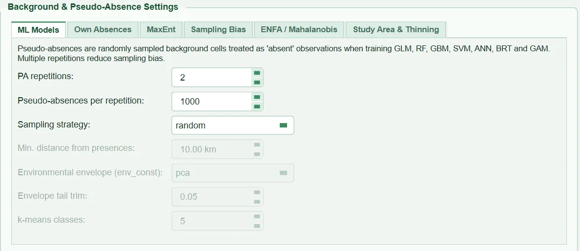
| Name in the UI | What it does | Default | Range / options | Code |
|---|---|---|---|---|
PA repetitions: |
Number of independent pseudo-absence sets | 2 | 1 – 10 | tabs/tab_data.py:293-297 |
Pseudo-absences per repetition: |
Number of pseudo-absences in each set | 1000 | 100 – 100,000 (step 500) | tabs/tab_data.py:299-304 |
Sampling strategy: |
Which cells the pseudo-absences are drawn from | random |
random, disk, sre, kmeans, env_const, geo_const, geo_env_const, geo_env_km_const |
tabs/tab_data.py:306-326, sdm_sampling.py:47-53 |
Min. distance from presences: |
Minimum distance to presences (km) | 10 km | 0 – 500 km | tabs/tab_data.py:328-333 |
Environmental envelope (env_const): |
How the envelope is built | pca |
pca, bioclim |
tabs/tab_data.py:335-342 |
Envelope tail trim: |
Proportion trimmed from each end of the envelope | 0.05 | 0.00 – 0.45 | tabs/tab_data.py:343-348 |
k-means classes: |
Number of clusters in environmental space | 5 | 2 – 30 | tabs/tab_data.py:349-353 |
Fields are enabled only for the strategy that uses them (tabs/tab_data.py:557-573): minimum distance for disk and geo_*; envelope and tail trim for env_const, geo_env_const, geo_env_km_const; k-means for kmeans, geo_env_km_const. If replace is selected in Own Absences, all fields are greyed out (§3.4).
3.3.1 PA repetitions
- What it does. With the same presences and a separately drawn set of
npseudo-absences each,PA repetitionstraining sets are built (sdm_core.py:3035-3082). The presence side of the sets is identical; only the absence side changes. ③ Models fits a separate model for each set (PA1,PA2in the log), and the ensemble combines the models from all sets (Chapters 5–6). - When and how to set it. The UI tooltip suggests 2–5. When working with few pseudo-absences (e.g. as many as there are presences), the number of repetitions should be increased; Barbet-Massin et al. (2012) recommend averaging 10 repetitions with as many pseudo-absences as presences for classification trees.
- Effect on results. Repetition turns a result that depends on the luck of a single draw into an average; the differences between sets show the uncertainty arising from the choice of pseudo-absences. Run time grows roughly in proportion to the number of repetitions.
- Caution. In
Own Absencesreplacemode the number of repetitions is reduced to 1, because there is no draw left to repeat (sdm_core.py:3031-3033); the report also states 1.
3.3.2 Pseudo-absences per repetition (number) and prevalence
- What it does. The number of pseudo-absences drawn in each set. Cells are drawn without replacement (
rng.choice(..., replace=False),sdm_core.py:2301-2302); if there are fewer candidate cells than requested, all are taken and a warning is written. - When and how to set it. The tooltip suggests the range 1000–10,000 and no fewer than the number of presences. Barbet-Massin et al. (2012) recommended a large number (e.g. 10,000) with equal weighting of presences and absences for regression methods (GLM, GAM), and many repetitions with as many pseudo-absences as presences for tree methods. In HABITUS, class weighting is set separately in ③ Models (Chapter 5).
- Effect on results. Prevalence (the proportion of presences in the training set) is determined by this number: p = n_{\text{presence}} / (n_{\text{presence}} + n_{\text{absence}}) (
sdm_core.py:3087-3089). In the example run it is 143/(143+1000) = 0.125. Prevalence directly changes the level of the raw output of unweighted models, and hence the threshold values: increasing the number of pseudo-absences lowers the raw probabilities. AUC is threshold-independent but sensitive to where the pseudo-absences come from (§3.3.3, §3.8). - Caution. If the number of pseudo-absences exceeds the number of valid cells in the accessible area, all cells in the area are used and the warning "The accessible area holds N usable cells, fewer than the M points requested" is written (
sdm_core.py:2190-2203). A point that falls on NoData in a predictor after sampling is dropped and counted ("PA1: N sampled point(s) fell on NoData…",sdm_core.py:2816-2841); because NoData cells of categorical layers are excluded from sampling in advance, this is rare.
3.3.3 Sampling strategy (eight strategies)
All strategies start from the same candidate set: cells that have a value in every continuous and categorical layer (_valid_cell_mask, sdm_core.py:2309-2330), restricted to those inside the accessible area if one is defined (sdm_core.py:2181-2203). The strategy-specific constraint is then applied (sdm_core.py:2205-2297), and the draw is made with bias and class weights, if any.
| Strategy | What it does | Fields used | R equivalent | Code |
|---|---|---|---|---|
random |
Equal-probability draw from candidate cells | — | biomod2 random, flexsdm random |
sdm_core.py:2291-2305 |
disk |
Excludes cells within Min. distance of each presence, draws randomly from the rest |
minimum distance | biomod2 disk (minimum distance only) |
sdm_core.py:2243-2258 |
sre |
Draws from cells outside the bioclimatic envelope of the presences; the envelope is the 5%–95% range of each variable at the presences | (fixed 0.05) | biomod2 sre |
sdm_core.py:2079-2119, 3005-3022 |
kmeans |
k-means in scaled environmental space; draws from classes containing no presences, with equal total weight per class | k | sdm eRandom, flexsdm kmeans |
sdm_sampling.py:245-288 |
env_const |
Draws from cells outside the environmental envelope of the presences | envelope, tail trim | flexsdm env_const |
sdm_sampling.py:219-242 |
geo_const |
Same rule as disk |
minimum distance | flexsdm geo_const |
sdm_sampling.py:26-27 |
geo_env_const |
Minimum distance and outside the envelope | minimum distance, envelope, tail trim | flexsdm geo_env_const |
sdm_core.py:2997-3003 |
geo_env_km_const |
Minimum distance, outside the envelope and presence-free k-means classes | all | flexsdm geo_env_km_const |
sdm_core.py:2399-2429 |
- What it does. The strategy determines "what" the model compares presences against.
randomrepresents the environmental variety of the accessible area as it is. The other strategies move pseudo-absences away from presences geographically (disk,geo_const) or environmentally (sre,env_const,kmeans); the aim is to reduce the labelling as "absent" of cells that are actually suitable but have no records (false absences). - When and how to set it. Barbet-Massin et al. (2012) recommended random selection for regression methods, and geographically and environmentally distant selection for classification trees and discriminant methods. The default
random, used together with an accessible area, is the option with the fewest assumptions. For an intensively sampled species with a high risk of false absences around the records,disk(e.g. 10–50 km) is a reasonable middle way. - Effect on results. Every constraint that moves pseudo-absences away from presences makes discrimination easier: AUC and TSS rise, but part of this rise is a product of the sampling design rather than of the model; response curves are cut off outside the presence range, and the suitable area on the map expands (VanDerWal et al. 2009; Barbet-Massin et al. 2012). The outside-envelope strategies (
sre,env_const) do this most strongly: the model tends to learn the inside of the envelope as "suitable" and the outside as "unsuitable", and simply reproduces the envelope. - Caution. The envelope and k-means strategies are computed with all continuous layers loaded in ① Data; because the selection in ② Variables is made later, unselected layers also affect where the pseudo-absences are placed. In
sre, a cell must be within range in all variables to count as inside the envelope; with 19 layers almost every cell falls outside in at least one variable, and the constraint weakens. If no cells remain outside the envelope, the strategy falls back to a random draw and a warning is written ("no cells outside the envelope found. Falling back to random sampling.";sdm_core.py:2206-2212). In strategies other thanrandom,diskandsre, if there are fewer candidate cells than requested, fewer points are drawn ("leaves only N candidate cells";sdm_core.py:2294-2297).
3.3.4 Min. distance from presences
- What it does. In
disk,geo_const,geo_env_constandgeo_env_km_const, the great-circle (haversine) distance from the centre of each candidate cell to each presence is computed; cells whose distance is not greater than this value are excluded (sdm_core.py:2243-2258). On a projected grid, the coordinates are first converted to longitude/latitude. - When and how to set it. A distance on the order of the location error of the records and the local spread of the species (a few km to a few tens of km) is a typical choice. Barbet-Massin et al. (2012) tested a distance of about 2° for classification methods; in a small study area this removes most candidates.
- Effect on results. As the distance grows, pseudo-absences move away from the presences and their environmental conditions; AUC/TSS rise, and the model draws a "wider" suitable area.
- Caution. With a distance of 0, the
geo_*strategies exclude nothing and report this as a warning (sdm_core.py:2999-3003). A very large distance stops with the error "No background cells remain after min_dist=… km. Reduce the minimum distance." The computation scans all candidate cells for each presence; on a global grid and with thousands of records it can take a long time.
3.3.5 Environmental envelope and Envelope tail trim
- What it does. In the
env_constfamily, the environmental envelope of the presences is built in one of two ways (sdm_core.py:2407-2420):pca: principal components (SVD) are computed on the standardised continuous variables in all valid cells; the [q,\,1-q] quantile range of the presences on the first two components forms the envelope. A cell is outside the envelope if it lies outside this range on at least one of the two components (sdm_sampling.py:219-242).bioclim: each variable separately; a cell is inside the envelope if it lies within the [q,\,1-q] range in all variables (the same computation assre, but q is adjustable;sdm_core.py:2410-2412).Envelope tail trimis q: 0 gives the full minimum–maximum range, 0.05 the 5%–95% range.
- When and how to set it.
pcais the closest to flexsdm'senv_constmethod. If location errors or outliers are suspected in the records, q is increased (the envelope narrows). - Effect on results. As q increases, the envelope narrows, the outside-envelope candidate area grows and the pseudo-absences approach presence conditions; as q decreases, the envelope widens, the pseudo-absences move environmentally away from the presences and discrimination becomes easier.
- Caution. The principal components are built from all valid cells, not restricted to the accessible area; the envelope itself is then intersected with the accessible area. The proportion of outside-envelope cells is written to the run record (
frac_cells_outside_envelope). Thesrestrategy does not use these two fields; its trim is always 0.05.
3.3.6 k-means classes
- What it does. Valid cells are split into
kclasses in standardised environmental space (scikit-learnKMeans,n_init=3; if there are more than 50,000 cells, the model is fitted on a random subsample of 50,000 cells and all cells are classified afterwards). Presences are assigned to the nearest class centre. Classes without presences are the source of pseudo-absences, and each receives the same total weight (stratified draw). If every class contains presences, the class weight becomes 1/(1+n_{\text{presence}}) and a warning is written (sdm_sampling.py:245-288). - When and how to set it. The default is 5. In an environmentally diverse study area, increasing the number of classes makes it easier to find presence-free classes.
- Effect on results. Equal class weights lead to over-representation of small but environmentally distinct classes among the pseudo-absences; environmental variety is balanced, but the geographic distribution changes.
- Caution. The classes are built from all valid cells; if all presence-free classes fall outside the accessible area, the run stops with the message "No candidate cell has a positive sampling weight" (
sdm_core.py:2281-2285). The k-means seed is derived from the run seed.
3.4 Your own absence records: Own Absences
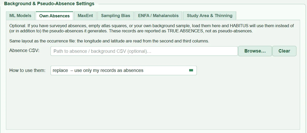
| Name in the UI | What it does | Default | Range / options | Code |
|---|---|---|---|---|
Absence CSV: + Browse… / Clear |
Observed absence (or own background) records; once selected, the record count and the columns to be read are previewed | empty | CSV | tabs/tab_data.py:478-491, 1162-1181 |
How to use them: |
Whether the records replace or supplement the pseudo-absences | replace |
replace – use only my records as absences / augment – my records plus generated pseudo-absences |
tabs/tab_data.py:493-507 |
3.4.1 Absence CSV and columns
- What it does. The file is read with the same reader as the records file (including delimiter and decimal detection). Coordinate columns are looked up in this order (
sdm_core.py:2729-2754): the longitude/latitude column names of the records file, if they also exist in this file; otherwiselongitude/lat…columns found by name; otherwise the 2nd and 3rd columns; if there are only two columns, the 1st and 2nd. Rows with empty coordinates are dropped and counted; those falling outside the raster or on NoData are dropped with the reason "absence record outside extent or on NoData", and if the loss exceeds 20%, an explanatory warning is given as for presences (sdm_core.py:2770-2797). - When and how to set it. For points where the species was not found in a field survey, empty atlas squares, or a target-group background compiled with the same method. These records are reported in the report and summary as "TRUE absences", separately from pseudo-absences.
- Effect on results. A model trained with true absences obtains the information "where the species does not occur" from observation rather than by guesswork; the meaning of the evaluation statistics also changes (discrimination against true absences rather than pseudo-absences).
- Caution. Absence records are not reduced to one per cell, not thinned, and not checked for falling in the same cell as a presence. If a file is given but cannot be used, the program does not silently fall back to pseudo-absences; it stops ("All N user-supplied absence records fall outside the raster extent…",
sdm_core.py:2791-2797).
3.4.2 replace and augment modes
- What it does.
replace: The absence side consists only of your records. No pseudo-absences are generated; all fields inML Modelsare greyed out, the number of repetitions drops to 1, and the minimum distance and accessible area are not applied to your records (tabs/tab_data.py:535-546,sdm_core.py:3031-3040).augment: Your records appear unchanged in each set, andPseudo-absences per repetitionpseudo-absences are drawn on top (sdm_core.py:3060-3062). The differences between sets come only from the generated part.
- When and how to set it.
replaceif the records come from a real and comprehensive absence survey;augmentif they are few, or a partial background rather than a complete survey. - Effect on results. In
replace, prevalence is your presence/absence ratio. Inaugment, the absence side grows and prevalence falls. - Caution. In
replacemode, if fewer than 20 absence records are supplied, the warning "Only N true absence records were supplied and pseudo-absences were switched off…" is given andaugmentis recommended (sdm_core.py:2807-2813). Absence records enter only the training sets of the two-class algorithms: MaxEnt continues to use its own background, and ENFA its own background (§3.5, §3.7).
3.5 MaxEnt background: MaxEnt
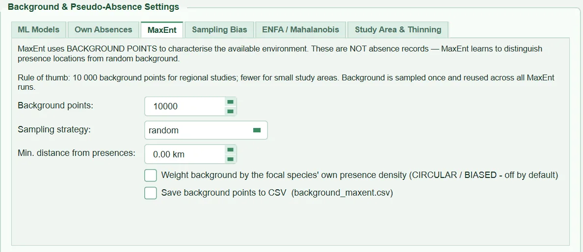
| Name in the UI | What it does | Default | Range / options | Code |
|---|---|---|---|---|
Background points: |
Number of MaxEnt background points | 10000 | 100 – 200,000 (step 1000) | tabs/tab_data.py:789-794 |
Sampling strategy: |
Draw rule | random |
random, disk |
tabs/tab_data.py:796-801 |
Min. distance from presences: |
Minimum distance to presences in disk |
0 km | 0 – 500 km | tabs/tab_data.py:803-806 |
Weight background by the focal species' own presence density (CIRCULAR / BIASED - off by default) |
Weights the background by the record density of the focal species | off | on / off | tabs/tab_data.py:808-822, sdm_core.py:3102-3142 |
Save background points to CSV (background_maxent.csv) |
Writes the background coordinates and predictor values | off | on / off | tabs/tab_data.py:824-830, 1549-1563 |
3.5.1 Background points and strategy
- What it does. The background is drawn once, separately from the pseudo-absences (
sdm_core.py:3144-3166); the accessible area and (if selected) target-group bias are applied. MaxEnt uses the whole of this background in every fit, including the cross-validation folds (sdm_core.py:4595-4603).diskis effective only ifMin. distanceis greater than 0; at 0 it is identical torandom. - When and how to set it. 10,000 is Maxent's common default (Phillips et al. 2006). If a small accessible area has fewer valid cells than this, all cells are used; the background is then a complete census of the area (Phillips and Dudík 2008).
- Effect on results. The size of the background determines how well the environmental distribution of the area is represented; the gain above 10,000 is usually small, while run time increases. The location of the background (accessible area) is far more influential than its size (§3.8).
- Caution. The background does not exclude presence cells; as in Maxent's definition, presences are also part of the available environment. The summary line "Background (MaxEnt): N points" gives the count after points dropped because of NoData have been subtracted.
3.5.2 Weighting by the focal species' own density (circular)
- What it does. When on, each valid cell is given as weight the sum of Gaussian kernels computed from its distances to all presences (bandwidth 0.5 units), and the background is drawn with this weight (
sdm_core.py:3119-3136). The background thus piles up where presences are dense. - When and how to set it. Not recommended; the box's name and tooltip say so explicitly. The focal species' own records carry both the bias and the species' true distribution; the weight cannot separate the two, and the model learns to ignore the environment of the best-sampled areas. A valid correction requires an independent bias surface (Phillips et al. 2009): the
Sampling Biassub-tab. - Effect on results. The contrast between presence and background decreases; AUC falls and response curves flatten.
- Caution. When switched on, the warning "MaxEnt background weighted by the focal species' own presence density: this is circular and biased…" is written to the log in every run. If a surface is given in
Sampling Biasand applied to MaxEnt, this box is ignored (sdm_core.py:3104-3107). The bandwidth is in raster coordinate units (0.5°, about 55 km, on a geographic grid).
3.6 Sampling bias: Sampling Bias
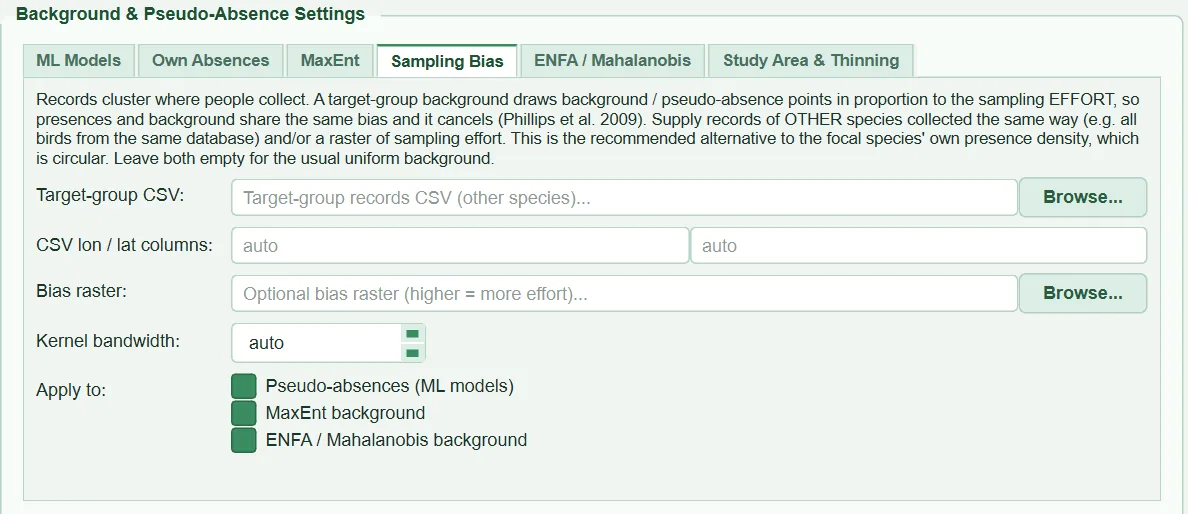
| Name in the UI | What it does | Default | Range / options | Code |
|---|---|---|---|---|
Target-group CSV: |
Records of other species collected with the same method | empty (off) | CSV | tabs/tab_data.py:402-405 |
CSV lon / lat columns: |
Coordinate columns in the target-group CSV | auto |
column name | tabs/tab_data.py:407-409, sdm_sampling.py:77-93 |
Bias raster: |
Sampling effort raster (large value = high effort) | empty (off) | .tif .tiff .img .asc |
tabs/tab_data.py:411-416, sdm_sampling.py:161-198 |
Kernel bandwidth: |
Gaussian smoothing (sigma) of the target-group density | auto (0) |
0 – 5000 km | tabs/tab_data.py:418-423, sdm_sampling.py:103-158 |
Apply to: |
Sets the surface is applied to | all three checked | Pseudo-absences (ML models), MaxEnt background, ENFA / Mahalanobis background |
tabs/tab_data.py:425-441, sdm_core.py:2991-2993 |
3.6.1 Target-group surface and bias raster
- What it does. Records concentrate where people collect them (around roads, villages, stations). The target-group approach (Phillips et al. 2009) draws the background and pseudo-absences in proportion to the record density of other species that carry the trace of the same effort; because presence and background carry the same bias, the bias cancels out. HABITUS builds a weight grid from two sources (
sdm_core.py:2332-2397):- Target-group CSV: records are counted into cells and smoothed with a Gaussian filter; the grid is divided by its maximum value, and cells with zero density are left a floor weight of 10^{-6} (
sdm_sampling.py:103-158). - Bias raster: read directly if on the same grid, otherwise resampled bilinearly; NaN, NoData and negative values become 0, and the grid is divided by its maximum value (
sdm_sampling.py:161-198). - If both are given, their product is used. The draw probability is proportional to the cell weight; the weight is combined with the accessible area and strategy constraints (multiplied by the k-means class weight;
sdm_core.py:2272-2289).
- Target-group CSV: records are counted into cells and smoothed with a Gaussian filter; the grid is divided by its maximum value, and cells with zero density are left a floor weight of 10^{-6} (
- When and how to set it. When sampling effort is clearly unbalanced. The target group should consist of species collected from the same database and with the same method as the focal species (e.g. all woody plant records of the same herbarium). The focal species' own records should not be placed in the target group; this would be circular.
- Effect on results. The background shifts towards accessible places; the model confuses "easy to reach" with "suitable" less often. AUC typically falls (discrimination becomes harder), but the map follows environmental conditions rather than roads and settlements (Kramer-Schadt et al. 2013).
- Caution. Target-group coordinates must be in the same coordinate system as the raster; if none fall on the grid, the run stops. With fewer than 20 target-group records a warning is written that the density will be very coarse, and when the surface is concentrated in less than 0.1% of the cells, a warning that most of the background will come from there (
sdm_core.py:2352-2393). A faulty file stops the run; the program does not silently fall back to uniform sampling. If the bias raster does not declare a coordinate system, it is assumed to be in the same system as the predictors and a warning is given; if its grid differs and it has no CRS, it cannot be aligned and an error is raised. When no surface is given, the note "Sampling bias: not corrected" is added to the report (sdm_core.py:1358-1363,2988-2990).
3.6.2 Kernel bandwidth
- What it does. The standard deviation (km) of the Gaussian smoothing. On a geographic grid, km is converted to degrees, corrected in the longitude direction by the cosine of the records' mean latitude. On a projected grid, km is converted using the metre equivalent of the map unit. With
auto(0), the normal reference rule is used for each axis: h = 1.06\,\min(s,\ \mathrm{IQR}/1.34)\,n^{-1/5} (MASSbandwidth.nrd/4, as inkde2d). Sigma is never smaller than one cell (sdm_sampling.py:136-154). - When and how to set it. Widened if the target-group records are sparse; kept at the level of a few cells if effort is concentrated right around roads.
- Effect on results. A small bandwidth sticks the surface to the record points, and the background comes almost only from recorded cells; a large bandwidth flattens the surface and brings it closer to uniform sampling.
- Caution. The bandwidth used is written to the run record (
auto (nrd)or km).
3.6.3 Apply to
The surface is applied only to the checked sets (sdm_core.py:2991-2993). Checking all three ensures that all algorithms see the same bias correction and makes comparisons between algorithms consistent. Checking only one is useful for testing the effect of the correction in a single family of algorithms.
3.7 ENFA background: ENFA / Mahalanobis
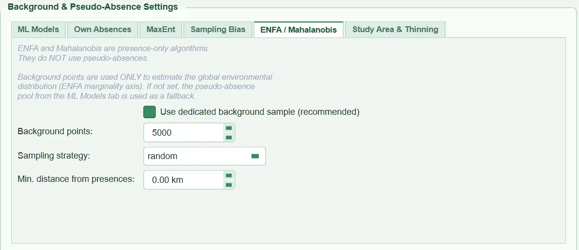
| Name in the UI | What it does | Default | Range / options | Code |
|---|---|---|---|---|
Use dedicated background sample (recommended) |
Draws a separate background for ENFA | on | on / off | tabs/tab_data.py:858-864 |
Background points: |
Number of background points | 5000 | 100 – 100,000 (step 1000) | tabs/tab_data.py:866-872 |
Sampling strategy: |
Draw rule | random |
random, disk |
tabs/tab_data.py:874-879 |
Min. distance from presences: |
Minimum distance in disk |
0 km | 0 – 500 km | tabs/tab_data.py:881-885 |
- What it does. ENFA compares the species' conditions with the "global" conditions of the study area: the global mean and covariance are computed from this background (
sdm_core.py:4079-4092). The background is drawn within the accessible area and (if checked) with the bias surface (sdm_core.py:3176-3199). If the box is off, ENFA computes the global statistics from the training rows (presences + pseudo-absences). - When and how to set it. Leaving it on is recommended: the global environment should be estimated from a uniform sample of the area, not from a sample distorted by the pseudo-absence strategy (e.g.
disk,sre). The tooltip considers 5000–10,000 points sufficient. - Effect on results. ENFA's marginality (deviation of the species' mean from the global mean) and specialisation axes are measured against this sample; narrowing the accessible area reduces marginality.
- Caution. In the code only ENFA uses this background; the Mahalanobis distance method uses only the mean and covariance of the presences (
sdm_core.py:4207-4230), and the settings of this tab do not change it. If the background columns do not exactly match the variables in the model, ENFA falls back to the training rows. Selectingdiskin the strategy box only activates the minimum distance.
3.8 Accessible area: Study Area & Thinning (upper half)
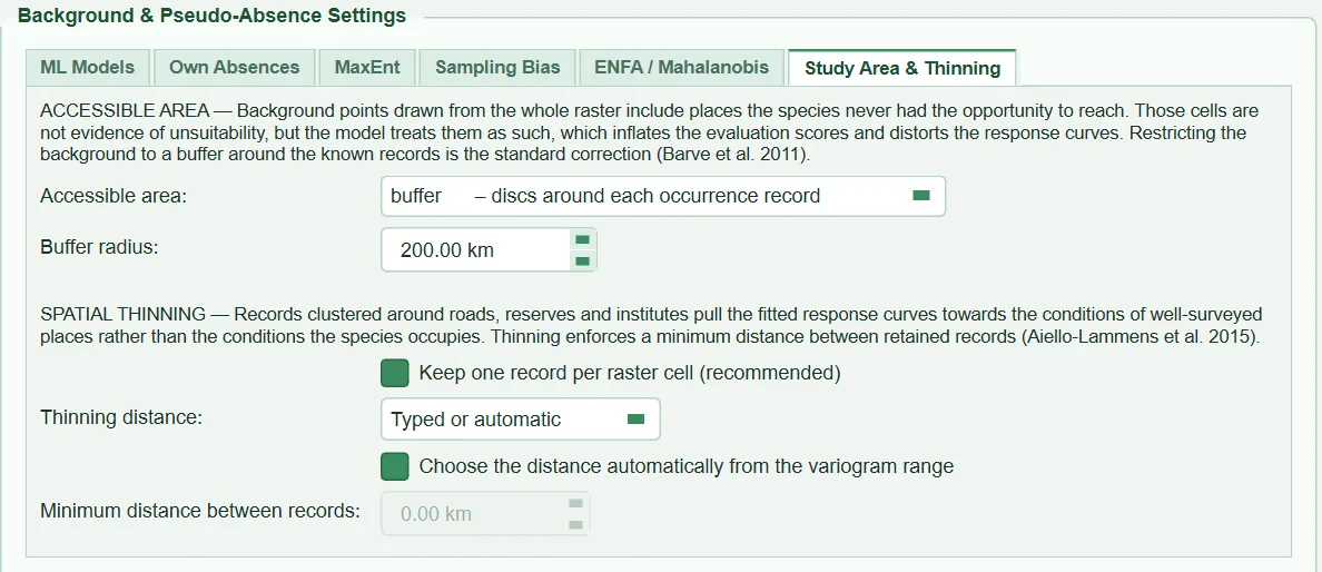
| Name in the UI | What it does | Default | Range / options | Code |
|---|---|---|---|---|
Accessible area: |
Method for building the background/pseudo-absence area | buffer |
buffer – discs around each occurrence record, mcp_buffer – buffered minimum convex polygon, polygon – my own calibration area layer, none – sample the whole raster extent |
tabs/tab_data.py:644-666 |
Buffer radius: |
Buffer radius; in polygon, the buffer added around the polygons |
200 km | 0 – 5000 km (step 50) | tabs/tab_data.py:668-674, 609-618 |
Calibration layer: + Browse… |
Calibration polygon layer (visible only in polygon) |
empty | .shp .gpkg .geojson .json .kml .gml |
tabs/tab_data.py:677-691 |
Keep only the polygons containing an occurrence record |
Keeps only polygons that contain records (only in polygon) |
on | on / off | tabs/tab_data.py:693-701 |
3.8.1 Why an accessible area
A species does not occur in places it has never been able to reach, even if they are suitable. These cells are not evidence of "unsuitable"; but when they enter the model as background or pseudo-absences, the model learns them as such (Barve et al. 2011). The accessible area (M in the BAM framework) restricts the area from which the background is drawn to the region the species can reach. Keeping the extent wide adds cells with conditions very different from the presences to the background; discrimination becomes easier and AUC rises artificially (Lobo et al. 2008; VanDerWal et al. 2009). The mask is applied to all three sets (pseudo-absences, MaxEnt, ENFA); it is not applied to the user's absence records. The map is still produced for the whole extent (or the study boundary).
3.8.2 Accessible area methods
- What it does.
buffer: All cells withinBuffer radiusof the cell of each presence (sdm_spatial.py:943-1062). Distance is computed with an anisotropic Euclidean distance transform (distance_transform_edt) that converts cell size to km; on a geographic grid, the cell width is reduced by the cosine of the records' mean latitude.mcp_buffer: The convex hull (minimum convex polygon) of the presence cells is filled, then the same buffer is added. If the records lie on a line (river, coast), the hull is the line segment between the two most distant records.polygon: The user's calibration layer (§3.8.4).none: No constraint; all valid cells.
- When and how to set it. Rojas-Soto et al. (2024) compared seven calibration-area methods on 31 species and recommended the method that uses biogeographic units (ecoregion, basin, biogeographic province); its counterpart in HABITUS is
polygon+Keep only the polygons containing an occurrence record. Buffer methods are safe and simple but cannot represent barriers (mountain ranges, sea).mcp_buffersuits species with continuous ranges; for fragmented ranges the hull also covers the gaps.noneshould be chosen only if the rasters have already been clipped to the area of interest. - Effect on results. As the area narrows, the background resembles presence conditions; AUC/TSS fall but become more honest, and response curves describe the gradient within M. In the example run, the 200 km buffer kept 40.0% of the raster extent.
- Caution. The buffer is built from the thinned records (
sdm_core.py:2971). Inbufferandmcp_buffer, a radius of 0 applies no constraint. If the buffer covers more than 97% of the extent, the warning "The accessible-area buffer covers almost the whole raster extent, so it is not constraining anything." is given (sdm_core.py:2694-2699). If the area has fewer cells than the number of points requested, all cells are used, a warning is written, and the draw is not extended to the whole extent (sdm_core.py:2166-2203). If the mask cannot be built, the program does not fall back to the whole extent; it stops.
3.8.3 Buffer radius
- What it does. In
bufferandmcp_buffer, the radius of M; inpolygon, the buffer added around the selected polygons (sdm_spatial.py:1260-1299). - When and how to set it. As the UI tooltip says, it should be chosen from the species' dispersal ability and the age of the range, not from the size of the raster. Tens of km for species with limited dispersal, hundreds of km for long-distance dispersers.
- Effect on results. As the radius grows, the background becomes environmentally more varied and AUC rises; prevalence does not change (the number of points is the same), but the pseudo-absences move away from the presences.
- Caution. When switching to
polygonmode, the field keeps the default value of 200 km; to use the polygons as drawn, the value must be reduced to 0 (tooltip: "Leave it at zero to use the polygon boundaries exactly as drawn"). The example run was run withbuffer200 km.
3.8.4 Calibration layer and "containing a record"
- What it does. The layer is read with pyogrio; only polygons are used. If its coordinate system differs from the rasters, it is reprojected; if the layer declares no system, it is assumed to be the same and a warning is given (
sdm_spatial.py:1194-1225). IfKeep only the polygons containing an occurrence recordis on, only polygons in which at least one presence falls are kept (biogeographic unit method); if off, all polygons in the layer are used. An optional buffer is added and the polygons are burned into the grid withall_touched=True(every cell touched by a polygon is inside) (sdm_spatial.py:1234-1321). The summary states "Calibration area: K of N polygons… X% of the raster extent". - When and how to set it. Loading an entire ecoregion layer without clipping and leaving the box on is the most practical way. If the layer contains only your study area, the box is switched off.
- Effect on results. M follows biogeographic boundaries; barriers that buffer methods cannot cross are taken into account.
- Caution. If no polygon contains a record, the run stops. With the box off, if no presence lies inside the polygons the warning "Calibration polygon: NONE of the N presence records lies inside the polygon(s)…" is given, and if fewer than 80% of presences lie inside, the warning "only K of N presence records… lie inside" (
sdm_core.py:2644-2672). Ifpolygonis selected and no layer is given, the run stops.
3.8.5 accessible_area.tif
If an accessible area is defined, the mask is written to the species' output folder as accessible_area.tif (1 = inside, 0 = outside, compressed uint8; tabs/tab_data.py:1536-1548, sdm_spatial.py:1065-1075). ⑥ Range Change uses this file to report change within this area separately (Chapter 9). If none is selected, the file is not written.
3.9 Thinning the records: Study Area & Thinning (lower half)
| Name in the UI | What it does | Default | Range / options | Code |
|---|---|---|---|---|
Keep one record per raster cell (recommended) |
One record in each predictor cell | on | on / off | tabs/tab_data.py:722-731 (Section 2.8.3) |
Thinning distance: |
Source of the thinning distance | Typed or automatic |
Typed or automatic, One cell, 10 km (Boria 2014) |
tabs/tab_data.py:733-743 |
Choose the distance automatically from the variogram range |
Chooses the distance from the variogram range (only in Typed or automatic) |
off | on / off | tabs/tab_data.py:745-751 |
Minimum distance between records: |
Manually entered distance (only in Typed or automatic with automatic off) |
0 km (no thinning) | 0 – 500 km | tabs/tab_data.py:753-765 |
3.9.1 How thinning works
- What it does. Records clustered around roads, protected areas and research institutions pull the response curves towards the conditions of well-sampled places rather than the conditions in which the species lives (Aiello-Lammens et al. 2015). Thinning enforces a minimum distance between any two retained records. The algorithm is greedy: records are visited in a seeded random order, and a record closer than the distance to an already retained record is dropped; this is tried with three different orders and the result retaining the most records is chosen (
sdm_spatial.py:888-937,sdm_core.py:2536). Distances are great-circle distances. - When and how to set it. Thinning is applied after the one-per-cell rule (Section 2.8.1). It is switched on if sampling is clearly clustered; if the records are already sparse and regular, it can stay off.
- Effect on results. The number of records drops, prevalence drops, and the remaining records are distributed more evenly in geographic space. Boria et al. (2014) showed that thinning reduces overfitting and improves performance in independent evaluation. Dropped records are listed with the reason "spatially thinned"; the distance used and how it was chosen are written to the log, summary, report and run record (
thinning.how_chosen). - Caution. By default spThin selects the largest set from many random repetitions; HABITUS's 3 repetitions approach this result but do not guarantee the largest set. If fewer than 10 records remain after thinning, a warning is given. If the manually entered distance is smaller than one cell, it is reported that it only separates records in neighbouring cells (
sdm_core.py:2526-2534).
3.9.2 Presets: One cell and 10 km
- What it does.
One cellsets the distance equal to the edge of a predictor cell: on a geographic grid, the mean of cell height × 110.57 km and cell width × 111.32 km × cos(mean latitude) (sdm_core.py:2554-2569).10 kmis the fixed distance used by Boria et al. (2014) and widely copied (sdm_core.py:2478-2483). When a preset is selected, the automatic box and the manually entered distance are greyed out. - When and how to set it.
One cellis the smallest meaningful distance, tied to predictor resolution, for separating records in neighbouring cells; with 2.5′ data it is about 4 km.10 kmis a convention, not a rule for every species and resolution. - Effect on results. Both are usually smaller than the automatic distance; they drop fewer records.
- Caution. The presets are not subject to the rule of retaining at least 50% of records.
3.9.3 Automatic distance: half the variogram range and the reduction rule
- What it does. In every run, even with thinning off, the program estimates the spatial autocorrelation range of the predictors from the record points (
sdm_spatial.py:166-281): at most 1500 records are subsampled; for each predictor an omnidirectional empirical semivariogram is computed in 15 bins up to half the maximum pairwise distance; the sill is the median semivariance of the outer third of the bins, and the range is the distance at which 95% of this sill is first reached; the median across variables is taken. With fewer than 20 points or no usable variogram, the range is taken as one tenth of the maximum distance (fallback_extent). With automatic thinning on, the distance is half the range; if this distance drops more than half of the records (THIN_MIN_RETAIN = 0.5), the distance is halved up to 8 times, and the first distance that retains at least 50% is used (sdm_core.py:2484-2522,2571-2594). - When and how to set it. If there is no species-specific justification for a distance, it is a defensible starting point; because the same range is used as the spatial block size in ③ Models, thinning and block size are consistent with each other (the logic of Roberts et al. 2017 and blockCV [Valavi et al. 2019]).
- Effect on results. In the example run the range was found to be 151.5 km; since its half, 75.7 km, would have dropped more than half of the records, the distance was reduced to 37.9 → 18.9 → 9.5 → 4.7 km; at 4.7 km, 143 of 221 records (65%) were retained (run record: "auto (half the variogram range, reduced to keep 65% of records)").
- Caution. In climate layers dominated by a regional trend, the range comes out very large and the reduction rule brings the distance down almost to the cell size; in this case the distance no longer removes autocorrelation, only clustering. If every candidate distance drops more than half of the records, no thinning is done and a warning is given; if the range cannot be computed at all, no thinning is done either and the message "Type a thinning distance in ① Data" is shown (
sdm_core.py:2495-2522). There is no 50% retention limit for a manually entered distance.
3.10 Outputs and what passes to the next step
pa_datasets:PA repetitionssets, each consisting of (predictor table, 0/1 labels, coordinates); passed to ③ Models.background_Xand its coordinates: the MaxEnt background; if requested,background_maxent.csv(columnslongitude, latitude, <variables>).background_ponly: the ENFA background.accessible_area.tifand accessible area information; thinning information; autocorrelation range (block size in ③).- The
background,study_areaandthinningsections of the run record: absence source (pseudo,user,user+pseudo), strategy and its details (candidate cell count, outside-envelope proportion, k-means class counts), background counts, target-group information, accessible area method and proportion, calibration polygons, thinning distance and how it was chosen. In the example run, settings left at their defaults are also listed underdefaults_left_unchanged.
3.11 Expert questions
Q1. Is the random pseudo-absence draw in HABITUS the same as random in biomod2?
Answer: The rule is the same: an equal-probability draw without replacement from valid cells (sdm_core.py:2301-2302). There are two differences. First, HABITUS by default restricts the draw to a 200 km accessible area; biomod2 has no such default and uses the whole extent. Second, pseudo-absences are drawn from cell centres, and within a set a cell is selected only once. Presence cells are not excluded in random; a pseudo-absence may fall in a presence cell.
Q2. Why do strategies that move pseudo-absences away from presences inflate the scores?
Answer: AUC and TSS measure the model's ability to discriminate presence from absence. When pseudo-absences are moved geographically (disk) or environmentally (sre, env_const) away from presences, discrimination becomes easier by construction of the data; the measured skill comes more from the sampling design than from the model (VanDerWal et al. 2009; Barbet-Massin et al. 2012). When comparing strategies on the same data, it is not the scores but the performance obtained with independent validation data (⑦ Validation) that should be compared.
Q3. Why is the accessible area buffer 200 km, and where does this value come from?
Answer: 200 km is a starting value (tabs/tab_data.py:669, sdm_core.py:1400); in the code it has no species-specific justification. The UI tooltip asks for the radius to be chosen from the species' dispersal ability and the age of the range. Barve et al. (2011) stress that M must be defined specifically for the species and the question; Rojas-Soto et al. (2024) recommend a calibration area based on biogeographic units (polygon in HABITUS). The value is written to the record in every run and should be reported.
Q4. Is the buffer distance computed geodesically?
Answer: No, it is computed approximately. buffer and mcp_buffer use an anisotropic Euclidean distance transform that treats cell height as constant and cell width as reduced by the cosine of the records' mean latitude (sdm_spatial.py:1022-1062). In areas with a small latitudinal span the error is small; for a range extending thousands of km north–south, the east–west width of the buffer deviates at the extremes. Thinning and minimum distance, by contrast, are computed with haversine.
Q5. Do the user's absence records also enter MaxEnt?
Answer: No. Own Absences records enter only the absence side of pa_datasets (sdm_core.py:3035-3082). MaxEnt uses its own background (sdm_core.py:4595-4598); the background is not treated as absence. ENFA also uses its own background. There is no path in the code for a user who wants to give true absences to MaxEnt as "background".
Q6. How is the bandwidth of the target-group surface chosen; what is its R equivalent?
Answer: With auto, 1.06\,\min(s,\ \mathrm{IQR}/1.34)\,n^{-1/5} is used for each axis; this is one quarter of the MASS bandwidth.nrd value and identical to the sigma that kde2d uses internally (sdm_sampling.py:143-151). The density is obtained by smoothing the cell counts with a Gaussian filter; mass beyond the boundary is lost (mode="constant"). The surface is scaled to its maximum value and floored at 10^{-6}, so that cells with no target records can still be selected, albeit with very low probability. Kramer-Schadt et al. (2013) and Phillips et al. (2009) give the rationale for this approach.
Q7. Why is the automatic thinning distance half the variogram range, and why is it reduced?
Answer: The range is the distance at which autocorrelation in the predictors vanishes; half of it is a common starting point for reducing repeated environmental information between records, and because the same range determines the block size, the two decisions are consistent (sdm_core.py:2433-2442). In climate layers with a strong regional trend the range comes out at hundreds of km and its half drops most of the records; since the aim of thinning is to remove redundancy, not the data set, the distance is halved until at least 50% of the records remain (sdm_core.py:2571-2594). In the example run it was reduced from 75.7 km to 4.7 km.
Q8. Does HABITUS's thinning give the same result as spThin?
Answer: The rule is the same (minimum distance between any two retained records, great-circle distance); the algorithm differs. spThin thin() performs many random repetitions and selects the set retaining the most records (Aiello-Lammens et al. 2015); HABITUS performs a greedy selection with 3 repetitions (sdm_spatial.py:888-937), and a single repetition in the automatic distance search. The number of retained records may be slightly lower than spThin's best; exact equality has not been tested.
Q9. What is the difference between sre and env_const (bioclim)?
Answer: Both use the same computation (_compute_sre_mask): the [q,\,1-q] range of the presences in each variable; a cell within range in all variables is inside the envelope (sdm_core.py:2079-2119). In sre, q is fixed at 0.05 (sdm_core.py:3010-3011); in env_const + bioclim it is set with Envelope tail trim. Variables with values at fewer than 4 presences are not included in the envelope. env_const + pca, by contrast, works on two principal components and prevents the envelope from becoming meaningless as the number of variables grows.
Q10. Do the background and pseudo-absences all come from the same seed; are the repetitions independent of each other?
Answer: DataFormatter sets up a single seeded generator and all draws are made from it in sequence (sdm_core.py:1505). Because each pseudo-absence set is drawn from the next state of the generator, the sets differ from each other and are reproduced with the same seed in the same order. Changing the number of repetitions also changes the subsequent MaxEnt and ENFA backgrounds, because the generator state has advanced.
Q11. What happens if the accessible area is small and has fewer cells than the requested number of background points?
Answer: All valid cells in the area are used, fewer points than requested are drawn and a warning is written (sdm_core.py:2190-2203); how many cells were found for which request is added to the run record (cells_short_of_request). The background is then a complete census of the area (Phillips and Dudík 2008). The draw is not extended to the whole extent; this preserves the M defined by the user.
Q12. Which settings on this tab affect the result most? Answer: No systematic sensitivity analysis has been carried out with the example data. From the structure of the code and the literature, the following order is expected: (1) accessible area method and radius (determines the environmental coverage of the background; Barve et al. 2011), (2) pseudo-absence strategy (determines the difficulty of discrimination; Barbet-Massin et al. 2012), (3) bias correction (determines whether the map follows bias or environment; Phillips et al. 2009), (4) thinning and the one-per-cell rule (determine the number of records used; from 626 to 143 in the example run). Pseudo-absence and background counts, within a reasonable range, are less influential.
3.12 Common mistakes and pitfalls
- Leaving
Buffer radiusat 200 km inpolygonmode: the polygons are expanded by 200 km. Enter 0 to use the polygons as they are. - Using a buffer even when the rasters are already clipped to the study area is not redundant; however, if the buffer covers more than 97% of the extent, the program reports this.
- Using the
geo_constordiskstrategy with 0 km: nothing is excluded. - Supplying the focal species' own records as the
Target-group CSV, or switching on the circular box in MaxEnt: the bias is not corrected but reinforced. - Supplying the target-group CSV in a coordinate system different from the rasters: "None of the N target-group points falls inside the raster extent."
replacewith few true absences: all threshold-dependent statistics become unstable; useaugment.- Comparing AUC/TSS across strategies and choosing the highest: the score difference comes from the design (Q2).
- Assuming that automatic thinning removes autocorrelation for every species: the reduction rule can make the distance very small; read the distance used from the summary.
- Assuming that the ENFA / Mahalanobis tab also changes Mahalanobis: only ENFA uses the background.
3.13 References
Aiello-Lammens, M.E., Boria, R.A., Radosavljevic, A., Vilela, B., Anderson, R.P., 2015. spThin: an R package for spatial thinning of species occurrence records for use in ecological niche models. Ecography 38, 541–545. https://doi.org/10.1111/ecog.01132
Barbet-Massin, M., Jiguet, F., Albert, C.H., Thuiller, W., 2012. Selecting pseudo-absences for species distribution models: how, where and how many? Methods in Ecology and Evolution 3, 327–338. https://doi.org/10.1111/j.2041-210X.2011.00172.x
Barve, N., Barve, V., Jiménez-Valverde, A., Lira-Noriega, A., Maher, S.P., Peterson, A.T., Soberón, J., Villalobos, F., 2011. The crucial role of the accessible area in ecological niche modeling and species distribution modeling. Ecological Modelling 222, 1810–1819. https://doi.org/10.1016/j.ecolmodel.2011.02.011
Boria, R.A., Olson, L.E., Goodman, S.M., Anderson, R.P., 2014. Spatial filtering to reduce sampling bias can improve the performance of ecological niche models. Ecological Modelling 275, 73–77. https://doi.org/10.1016/j.ecolmodel.2013.12.012
Kramer-Schadt, S., Niedballa, J., Pilgrim, J.D., Schröder, B., Lindenborn, J., Reinfelder, V., Stillfried, M., Heckmann, I., Scharf, A.K., Augeri, D.M., Cheyne, S.M., Hearn, A.J., Ross, J., Macdonald, D.W., Mathai, J., Eaton, J., Marshall, A.J., Semiadi, G., Rustam, R., Bernard, H., Alfred, R., Samejima, H., Duckworth, J.W., Breitenmoser-Wuersten, C., Belant, J.L., Hofer, H., Wilting, A., 2013. The importance of correcting for sampling bias in MaxEnt species distribution models. Diversity and Distributions 19, 1366–1379. https://doi.org/10.1111/ddi.12096
Lobo, J.M., Jiménez-Valverde, A., Real, R., 2008. AUC: a misleading measure of the performance of predictive distribution models. Global Ecology and Biogeography 17, 145–151. https://doi.org/10.1111/j.1466-8238.2007.00358.x
Phillips, S.J., Anderson, R.P., Schapire, R.E., 2006. Maximum entropy modeling of species geographic distributions. Ecological Modelling 190, 231–259. https://doi.org/10.1016/j.ecolmodel.2005.03.026
Phillips, S.J., Dudík, M., 2008. Modeling of species distributions with Maxent: new extensions and a comprehensive evaluation. Ecography 31, 161–175. https://doi.org/10.1111/j.0906-7590.2008.5203.x
Phillips, S.J., Dudík, M., Elith, J., Graham, C.H., Lehmann, A., Leathwick, J., Ferrier, S., 2009. Sample selection bias and presence-only distribution models: implications for background and pseudo-absence data. Ecological Applications 19, 181–197. https://doi.org/10.1890/07-2153.1
Roberts, D.R., Bahn, V., Ciuti, S., Boyce, M.S., Elith, J., Guillera-Arroita, G., Hauenstein, S., Lahoz-Monfort, J.J., Schröder, B., Thuiller, W., Warton, D.I., Wintle, B.A., Hartig, F., Dormann, C.F., 2017. Cross-validation strategies for data with temporal, spatial, hierarchical, or phylogenetic structure. Ecography 40, 913–929. https://doi.org/10.1111/ecog.02881
Rojas-Soto, O., Forero-Rodríguez, J.S., Galindo-Cruz, A., Mota-Vargas, C., Parra-Henao, K.D., Peña-Peniche, A., Piña-Torres, J., Rojas-Herrera, K., Sánchez-Rodríguez, J.D., Toro-Cardona, F.A., Trinidad-Domínguez, C.D., 2024. Calibration areas in ecological niche and species distribution modelling: Unravelling approaches and concepts. Journal of Biogeography 51, 1416–1428. https://doi.org/10.1111/jbi.14834
Valavi, R., Elith, J., Lahoz-Monfort, J.J., Guillera-Arroita, G., 2019. blockCV: An R package for generating spatially or environmentally separated folds for k-fold cross-validation of species distribution models. Methods in Ecology and Evolution 10, 225–232. https://doi.org/10.1111/2041-210X.13107
VanDerWal, J., Shoo, L.P., Graham, C., Williams, S.E., 2009. Selecting pseudo-absence data for presence-only distribution modeling: How far should you stray from what you know? Ecological Modelling 220, 589–594. https://doi.org/10.1016/j.ecolmodel.2008.11.010