4. Variables (② Variables)
Tab: ② Variables · Code: tabs/tab_vif.py (VIF + Correlation), tabs/tab_vif_advanced.py (Advanced Analysis), sdm_core.py compute_vif, compute_correlation_matrix, variable_priority_ranking (computation)
4.1 What this tab does
② Variables shows the collinearity among the continuous predictors loaded in the ① Data step (collinearity: a predictor being close to a linear combination of the other predictors) and lets the user select the variables that will enter the model. The selection is made by the user. The program only ranks, flags and offers a starting suggestion (Recommended); no variable leaves the model without confirmation.
- Input: the pseudo-absence (PA) sets produced by ① Data (
state["pa_datasets"]) and the names of the continuous variables (formatter.var_names). Categorical rasters are listed in a separate section; they do not enter the VIF or the correlation. - Output: the selected continuous variables (
state["var_names"]), the selected and excluded categorical rasters (state["cat_selected"],state["cat_excluded"]), and four files written underfigures/(§4.8). - Lock order: the tab opens once ① Data is complete. The
Confirm Variable Selection → Proceed to ③ Modelsbutton unlocks the ③ Models tab and switches to it (tabs/tab_vif.py:1206-1208).
The tab has two sub-tabs: VIF + Correlation (where the selection is made) and Advanced Analysis (complementary diagnostics with the condition number, principal components, LASSO and Ridge). The second sub-tab does not make a selection; it only provides information.
4.2 Screen layout
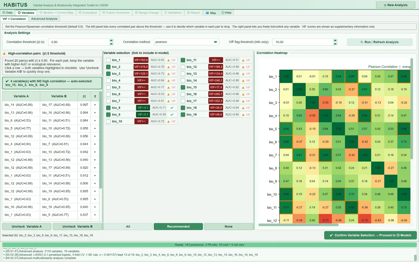
Figure 4.1 is taken from the example run (Abies nordmanniana, 143 presences used, 2 PA sets × 1000 points, 19 WorldClim bioclimatic variables). Regions:
| Region | What it contains | Subsection |
|---|---|---|
Top information strip and Analysis Settings |
Correlation threshold, correlation method, VIF threshold, Run / Refresh Analysis |
§4.4 |
Left panel High-correlation pairs (|r| ≥ threshold) |
Table of pairs exceeding the threshold, "safe" variable box, Uncheck Variable A/B |
§4.5 |
Middle panel Variable selection (tick to include in model) |
For each continuous variable a checkbox, VIF badge, AUC badge and status icon; the categorical section below it; All, Recommended, None |
§4.6 |
Right panel Correlation Heatmap |
Correlation matrix with square cells; cells exceeding the threshold have an orange border | §4.5.3 |
| Bottom strip | Selection summary ("Selected (n): …") and Confirm Variable Selection → Proceed to ③ Models |
§4.7 |
Advanced Analysis sub-tab |
Condition Number, PCA, LASSO (L1), Ridge (L2) |
§4.9 |
4.3 Which sample the computations use
All numbers in this tab are computed on a sample, not on all raster cells. The sample is the PA sets produced by ① Data stacked on top of each other: each set contains all presences used plus the pseudo-absences of that set (tabs/tab_vif.py:349-353, sdm_core.py:3221-3226). In the example run this gives 2 × (143 + 1000) = 2286 rows. The MaxEnt background points (10,000) do not enter this pool.
The two sub-tabs prepare the pool differently:
VIF + Correlationuses the pool as it is; it only drops rows with missing values (dropna). Each presence appears as many times as there are PA sets (twice in the example).Advanced Analysisdrops duplicate rows: presences that are identical in every PA set are counted once, and pseudo-absences that happen to fall in the same cell in two sets are also deduplicated (tabs/tab_vif_advanced.py:356-363). In the example run 2110 rows remain (status line in Figure 4.2: "2110 samples × 19 variables").
Note: VIF and correlation describe the relationships among the predictors themselves; they do not look at the presence/absence label. They do, however, depend on the points at which they are measured. If the accessible area (① Data) is kept large, the pseudo-absences spread over a wider climatic range and the correlations may change. The correlation of the same layers over the whole study area need not be the same as the correlation in this sample.
The univariate AUC (below), by contrast, does look at the label: presences are taken as 1 and pseudo-absences as 0.
4.4 Analysis settings (Analysis Settings)
This strip determines the thresholds with which the pairs table, the heatmap and the Recommended suggestion are built.
| Name in the UI | What it does | Default | Range / options | Code |
|---|---|---|---|---|
Correlation threshold (|r| ≥): |
Lists pairs whose absolute correlation is equal to or greater than this value and frames them in the heatmap; used in the second step of Recommended |
0.80 | 0.30–0.99, step 0.05 | tabs/tab_vif.py:123-130, sdm_core.py:435-445 |
Correlation method: |
Pearson (linear) or Spearman (rank) correlation | pearson |
pearson, spearman |
tabs/tab_vif.py:132-136, sdm_core.py:300-302 |
VIF flag threshold (info only): |
Badge colouring, the VIF_OK flag and the stepwise VIF threshold of Recommended |
10.00 | 2–50, step 1 | tabs/tab_vif.py:138-143, sdm_core.py:405, sdm_core.py:427-434 |
↻ Run / Refresh Analysis |
Recomputes the ranking, pairs, list and heatmap with the three values above | — | button | tabs/tab_vif.py:339-376 |
4.4.1 Correlation threshold (Correlation threshold)
- What it does. Writes every pair with |r| \ge threshold in the upper triangle of the correlation matrix to the left table, sorts them by |r| in descending order (
tabs/tab_vif.py:696-705) and marks these cells with an orange border in the heatmap (tabs/tab_vif.py:984-991). Variables that appear in no pair are counted as "safe" (§4.5.2). Together withRun / Refresh Analysis, it also determines the correlation step ofRecommended(§4.6.2). - When and how to set it. The tooltip gives three common values: 0.70 (conservative), 0.80 (default), 0.90 (lenient). In simulation studies, Dormann et al. (2013) report that |r| > 0.7 is the approximate limit at which collinearity begins to seriously distort model estimation and prediction. If the model is to be transferred to another region or climate (future scenario), 0.70 is safer; if only the description of the current distribution is required, 0.80 is often sufficient.
- Effect on results. As the threshold decreases, the number of pairs increases, the number of safe variables decreases and
Recommendedretains fewer variables. In the example run, 20 pairs are listed with the 0.80 threshold (Figure 4.1; the strongest pair is bio_14–bio_17, |r| = 0.997). - Caution. Changing the value in the box refreshes the pairs table and the heatmap immediately (
tabs/tab_vif.py:880-884), but it does not refresh theRecommendedsuggestion or theCorr_OKflag; for these,Run / Refresh Analysismust be pressed. The suggestion shown when the tab first opens comes from the automatic pre-computation of the ① Data step, and this pre-computation uses a threshold of 0.70, the Pearson method and a VIF threshold of 10 (sdm_core.py:3225-3227,sdm_core.py:305-309), whereas the box shows 0.80. For a suggestion computed with the values in the UI, pressRun / Refresh Analysisfirst.
4.4.2 Correlation method (Correlation method)
- What it does. Computes the Pearson or Spearman matrix with
pandas.DataFrame.corr(method=…)(sdm_core.py:300-302). The pairs table, the heatmap, the mean absolute correlation (Mean_Corr) and the correlation step ofRecommendeduse this matrix. VIF is not affected by this choice; VIF is always computed by linear regression. - When and how to set it. Tooltip: "pearson: linear correlation (assumes normality)", "spearman: rank-based, robust to non-normality and outliers". Spearman is more appropriate for predictors with skewed distributions, such as precipitation variables, or with monotonic but non-linear relationships.
- Effect on results. Because Spearman also captures monotonic non-linear relationships, it usually lists more pairs. Since the VIF step does not change, the first stage of
Recommendedstays the same. - Caution. Nothing is refreshed automatically when the method box is changed (no signal is connected to the box,
tabs/tab_vif.py:132-136);Run / Refresh Analysismust be pressed.
4.4.3 VIF threshold (VIF flag threshold (info only))
- What it does. It is used in three places: (1) the VIF badge in the variable list is red if the value exceeds the threshold and green otherwise (
tabs/tab_vif.py:443-462); (2) theVIF_OKflag is true when \text{VIF} \le threshold and \text{VIF} < 999 (sdm_core.py:405); (3) afterRun / Refresh Analysis, the stepwise VIF stage ofRecommendedremoves variables down to this threshold (sdm_core.py:427-434,tabs/tab_vif.py:357). - When and how to set it. 10 is the commonly used limit; the default of usdm::vifstep is also
th = 10. O'Brien (2007) argues that such thresholds should be read not as rules but as signals to be weighed together with sample size and purpose. For models whose coefficients will be interpreted, such as GLM and GAM, a stricter threshold such as 5 may be considered. - Effect on results. As the threshold decreases,
Recommendedretains fewer variables. It does not remove variables by itself: the ticks in the list do not change; the new suggestion is applied only when theRecommendedbutton is pressed. - Caution. The phrase "(info only)" in the UI and the sentence "does NOT force deselection" in the tooltip mean that the threshold does not forcibly remove any variable. The threshold nevertheless determines the
Recommendedsuggestion. Changing the value in the box does not refresh anything on its own;Run / Refresh Analysisis required.
4.4.4 How VIF is computed
Each continuous variable x_i is regressed on all the other continuous variables by linear regression with an intercept (sklearn.linear_model.LinearRegression), and
is computed (sdm_core.py:221-297). Details:
- Only rows in which x_i and all the other variables are finite are used; if there are fewer than 10 such rows or the variable is constant, the result is
NaNand the badge showsVIF=—(sdm_core.py:269-282). - R^2 is clipped to the [0, 1] interval to guard against floating-point overflow. If R^2 > 0.9999 (true VIF above 10,000), the value is capped at 999 and the badge shows
VIF=∞(sdm_core.py:286-295,tabs/tab_vif.py:447-451). This is normal for WorldClim variables derived from one another (e.g. bio_7 = bio_5 − bio_6). - At least two variables are required; with a single variable VIF is undefined and the ranking table writes VIF = 1 for each variable (
sdm_core.py:356-368).
4.5 Highly correlated pairs and the heatmap
The left panel and the heatmap on the right are built from the same correlation matrix. The aim is to show pairs of variables that substitute for each other and to make it easier for the user to decide which member of each pair to keep.
| Name in the UI | What it does | Default | Range / options | Code |
|---|---|---|---|---|
Pairs table (Variable A, Variable B, |r|, ±) |
Each pair exceeding the threshold; univariate AUC next to the name; absolute r and sign | — | — | tabs/tab_vif.py:682-801 |
| Clicking a pair row | Highlights the frames of the two variables in the list in orange and scrolls them into view | — | — | tabs/tab_vif.py:827-865 |
Uncheck Variable A / Uncheck Variable B |
Unticks the first / second variable of the selected pair | — | button | tabs/tab_vif.py:209-221, 867-878 |
| Safe variable box | Variables that appear in no pair ("auto-selected") | — | — | tabs/tab_vif.py:707-729 |
Correlation Heatmap |
Matrix with square cells; RdYlGn colour scale, −1…+1 | — | — | tabs/tab_vif.py:937-1009 |
4.5.1 Columns of the pairs table
Variable A,Variable B: the two variables of the pair, in their natural order in the matrix (bio_1 first, bio_10 after). The univariate AUC of the variable is shown in parentheses next to its name, and of the two variables the one with the lower AUC is shown in red and the one with the higher AUC in green (tabs/tab_vif.py:752-772).|r|: absolute correlation, three decimals. Colour: \ge 0.95 red, \ge 0.85 orange, below that neutral (tabs/tab_vif.py:777-785).±: sign of the correlation (+or−).
The information text above the panel gives the number of pairs ("Found 20 pair(s) with |r| ≥ 0.80"). If there are no pairs, it reads "No variable pairs exceed |r| ≥ … All variables can be safely used together."
Caution: The AUC colouring of the pairs table and the advice "keep the variable with higher AUC or ecological relevance" in the information text are not the same as the criterion of
Recommended:Recommendedremoves the member of a pair with the higher VIF and does not look at AUC (§4.6.2). The univariate AUC is for information only; a variable that discriminates well in this sample may be doing so because of its correlation with the true driver and may fail when transferred (sdm_core.py:323-339). Which member of a pair to keep should be decided primarily by the ecology of the species.
4.5.2 Safe variables
Variables that appear in no pair exceeding the threshold are listed in a green box under the heading "N variable(s) with NO high correlation — auto-selected". When the list is rebuilt, these variables always come ticked (tabs/tab_vif.py:427-431). In the example run, four variables are safe with the 0.80 threshold: bio_15, bio_3, bio_8, bio_9 (Figure 4.1).
Note: "Safe" refers only to pairwise correlation. A variable may be close to a combination of several variables without being strongly related to any single one; VIF shows this. In the example, bio_3 is in no pair, but its VIF in the full set is 125.1.
Recommendeddoes not add the safe variables automatically; it only applies the result of the stepwise selection (tabs/tab_vif.py:900-915).
4.5.3 Correlation heatmap
The heatmap shows the matrix of all continuous variables computed with the selected method. Cells are square and of fixed size (0.5 inch for up to 25 variables, 0.4 inch for more); a large matrix is not compressed but navigated with a scroll bar (tabs/tab_vif.py:953-963). For up to 25 variables, cell values are printed with two decimals. Off-diagonal cells exceeding the threshold have an orange border; the title has the form "Pearson Correlation | orange border = |r| ≥ 0.80". At every redraw the figure is saved as figures/correlation_heatmap.png at 300 dpi (if an output folder is defined; tabs/tab_vif.py:1006-1009).
4.6 Variable list and bulk selection
The list in the middle panel is where the continuous variables that will enter the model are selected. If there are more than 12 variables, it is split into two columns (tabs/tab_vif.py:522-528).
| Name in the UI | What it does | Default | Range / options | Code |
|---|---|---|---|---|
| Variable checkbox | A ticked variable enters the model | safe variables and the Recommended suggestion ticked |
on / off | tabs/tab_vif.py:423-438 |
| VIF badge | VIF in the full set; green ≤ threshold, red > threshold, VIF=∞ capped, VIF=— could not be computed |
— | — | tabs/tab_vif.py:441-469 |
| AUC badge | Univariate AUC; neutral colour, information only | — | 0.5–1 | tabs/tab_vif.py:471-499, sdm_core.py:380-393 |
| Status icon | ⚠ VIF (VIF_OK false), ⚠ Corr (Corr_OK false), ✔ (recommended), – |
— | — | tabs/tab_vif.py:501-517 |
All |
Ticks all continuous variables | — | button | tabs/tab_vif.py:890-893 |
Recommended |
Applies the result of the stepwise selection and writes the removals to the log | — | button | tabs/tab_vif.py:900-915 |
None |
Unticks all continuous variables | — | button | tabs/tab_vif.py:895-898 |
4.6.1 Priority table and its columns
variable_priority_ranking produces one row per variable; the list badges are read from this table, and on confirmation the table is written as figures/variable_priority_ranking.csv (sdm_core.py:305-465, tabs/tab_vif.py:1083-1096). Rows are sorted by Priority_Score in descending order.
| Column | Meaning |
|---|---|
Variable |
Variable name |
VIF |
VIF in the full set (two decimals; 999 = capped) |
Mean_Corr |
Mean absolute correlation with the other variables (diagonal taken as 0) |
Univariate_AUC |
Ability of the variable on its own to separate presences from pseudo-absences; if below 0.5, 1 - \text{AUC} is taken |
Priority_Score |
0.5\,(1 - (\min(\text{VIF}, 50) - 1)/49) + 0.5\,(1 - \text{Mean\_Corr}), clipped to [0, 1] |
VIF_OK |
\text{VIF} \le threshold and \text{VIF} < 999 |
Corr_OK |
Mean_Corr < correlation threshold |
Recommended |
Whether it survived the stepwise selection |
VIF_in_selection |
VIF within the recommended set (empty for variables not recommended) |
Priority_Score is based only on collinearity; the univariate AUC sits in the table as information but does not enter the ranking as a weight (sdm_core.py:395-401). The rationale is explicit in the code: promoting a predictor that discriminates well in this sample would be a selection that ignores ecological meaning and transferability to another region or climate.
Note:
Corr_OKlooks not at individual pairs but at the mean absolute correlation of the variable. In the example run, with the 0.70 threshold,Corr_OKis true for all 19 variables (the highestMean_Corris 0.533, for bio_12), whereas 20 pairs exceed 0.80. This is why the⚠ Corricon is rarely seen; pairs are shown by the left table.
4.6.2 Recommended selection (Recommended): stepwise VIF and correlated pairs
-
What it does. The
Recommendedbutton applies theRecommendedcolumn ofvariable_priority_rankingto the list; it leaves no other variable ticked (tabs/tab_vif.py:907-909). This column is obtained through a two-stage procedure (sdm_core.py:427-447):- Stepwise VIF. Start with all continuous variables. The VIFs of the remaining set are recomputed; if the largest VIF exceeds the threshold, that variable is removed. Stop when the largest VIF is equal to or below the threshold, or when a single variable remains.
- Correlated pair. Among the remaining variables, the strongest of the pairs with |r| \ge correlation threshold is found; of the two members of the pair, the one with the larger VIF in the remaining set is removed (the first one if tied). This continues until no such pair remains.
Each removed variable is written to the log in order, with its VIF or |r| value at the moment of removal.
-
When and how to set it. It is used as a starting point. The tooltip says so too: "A starting point: check it against what you know of the species." First set the thresholds, press
Run / Refresh Analysis, then pressRecommendedand correct the result manually according to the ecology of the species (for example, keeping the ecologically more meaningful member of a pair). - Effect on results. In the example run the stepwise selection removed 11 variables in this order: bio_4 (VIF 999), bio_5 (999), bio_1 (757.27), bio_7 (653.22), bio_17 (346.39), bio_16 (236.16), bio_6 (130.1), bio_12 (80.89), bio_10 (74.4), bio_14 (26.21), bio_13 (15.98). The remaining eight variables are bio_2, bio_3, bio_8, bio_9, bio_11, bio_15, bio_18, bio_19; the VIFs within this set range from 1.65 (bio_15) to 6.43 (bio_18), and since no pair exceeding the correlation threshold remained among them, the second stage removed nothing (
_calisma/figures/variable_priority_ranking.csv, session log). In the full set only two variables (bio_8 and bio_9) have a VIF below 10; filtering by full-set VIF would therefore leave very few variables. The stepwise method avoids this problem. - Caution. The stepwise method works not on the VIF in the full set but on the VIF recomputed at each step. A variable showing
VIF=∞in the full set (bio_11 in the example) can therefore remain in the recommended set; the badge in the list describes the full set, theVIF_in_selectioncolumn the recommended set. When capped values (999) are tied, the first variable in natural order is removed (v_now.idxmax(),sdm_core.py:430); in this case the removal order may differ from that of a computation that does not cap VIF (§4.11, Q2).
Same result as usdm::vifstep
The stepwise VIF stage does what the vifstep function of the R package usdm (Naimi et al. 2014) does. For this book the two were compared on the same matrix: 19 WorldClim 2.1 bioclimatic variables at 5000 land cells drawn at random within the study extent (10° W–50° E, 30–46° N); variable_priority_ranking(..., vif_threshold=10) in HABITUS, usdm::vifstep(d, th = 10) in R (script: habitus_dogrulama\H3_yazilim_tanitim\betikler\Y10_vif_usdm.py). The two programs removed 11 variables in the same order (bio_5, bio_10, bio_11, bio_16, bio_7, bio_17, bio_1, bio_12, bio_3, bio_13, bio_18), and the VIFs of the remaining eight variables agree to the fourteenth decimal:
| Variable | usdm::vifstep VIF | HABITUS VIF |
|---|---|---|
| bio_2 | 2.375571 | 2.375571 |
| bio_4 | 2.524650 | 2.524650 |
| bio_6 | 6.864633 | 6.864633 |
| bio_8 | 2.787451 | 2.787451 |
| bio_9 | 6.130096 | 6.130096 |
| bio_14 | 3.548789 | 3.548789 |
| bio_15 | 3.131781 | 3.131781 |
| bio_19 | 2.161437 | 2.161437 |
(Source: habitus_dogrulama\H3_yazilim_tanitim\yazim\dogrulama_vif_usdm.csv; the table is rounded to six decimals.) In the comparison the correlation threshold was kept at 0.99, i.e. the second stage was disabled; usdm has no counterpart of this stage (usdm::vifcor applies correlation first and with a different rule).
4.6.3 Univariate AUC
For each variable sklearn.metrics.roc_auc_score(y, x) is computed; if it is below 0.5, the relationship is treated as reversed and 1 - \text{AUC} is written (sdm_core.py:380-393). If there are fewer than 10 valid rows or the computation fails, 0.5 is written. The badge is deliberately neutral in colour: a low AUC is not a reason to remove a variable (tabs/tab_vif.py:471-499). In the example run the highest values are for precipitation variables (bio_12 0.887; bio_17 0.886) and the lowest for temperature variables (bio_11 0.51; bio_6 0.533).
4.6.4 Categorical variable section
If the data contain categorical rasters, a fixed box titled Categorical variables (not part of VIF) opens below the list (tabs/tab_vif.py:557-671). Each categorical raster is one row:
| Item | What it does | Default | Code |
|---|---|---|---|
| Checkbox | A ticked raster enters the model | ticked (or the previous confirmation, if any) | tabs/tab_vif.py:602-616 |
Class badge (N classes) |
Number of classes; the tooltip gives "presences / records" per class (first PA set) | — | tabs/tab_vif.py:618-639 |
| Class count text | "class:presences/records" values of the first four classes | — | tabs/tab_vif.py:641-651 |
| Sparse class warning | Number of classes with fewer than 3 presences ("⚠ k classes <3 presences") | — | tabs/tab_vif.py:653-664, sdm_core.py:1264 |
Categorical rasters do not enter the VIF or the correlation; All, Recommended and None do not touch this box. The tooltip states how each algorithm uses a categorical variable: GLM, GLMNET, SVM and ANN through dummy (one-hot) columns; GAM through a factor term; MaxEnt through the categorical feature class; tree-based methods through integer splits; BIOCLIM, Domain, ENFA, Mahalanobis and ESM use only continuous variables (tabs/tab_vif.py:536-545). If records were dropped in ① Data solely because of the NoData of one raster, the tooltip reports this with the counts and notes that excluding the raster does not redo the sampling. The example run has no categorical raster, so the box is not shown.
4.7 Confirmation (Confirm) and the records-per-predictor check
| Name in the UI | What it does | Default | Code |
|---|---|---|---|
✔ Confirm Variable Selection → Proceed to ③ Models |
Saves the selection, writes the files, unlocks ③ Models | — | tabs/tab_vif.py:1160-1225 |
4.7.1 Confirmation
- What it does. Writes the ticked continuous variables in natural order to
state["var_names"], the categorical selection tostate["cat_selected"]and the excluded ones tostate["cat_excluded"](tabs/tab_vif.py:1187-1191). The order in which variables are ticked does not matter; the selection is always sorted by natural name order (sdm_core.canonical_order). It then writes the files in §4.8, unlocks ③ Models and switches to itsAlgorithm Settingssub-tab. - When and how to set it. Press it once when the selection is finished. If the selection is changed later, it must be pressed again; otherwise ③ Models uses the old selection.
- Effect on results. All subsequent steps (models, future projections, novelty maps) use only the confirmed variables.
- Caution. At least two continuous variables are required: if nothing is selected, the message "Please select at least one variable." appears; with a single variable, "At least 2 variables are needed for modelling. Please select more variables." appears (
tabs/tab_vif.py:1162-1167). If models have already been run, the "Re-confirm Variable Selection" dialog states that confirming will delete all models, maps, projections and evaluation results; ifYesis chosen, these are deleted (tabs/tab_vif.py:1170-1185,main_dialog.py:528-542).
4.7.2 Records-per-predictor check
After confirmation the program divides the number of presences used by the number of selected predictors (continuous + categorical) (sdm_core.py:2889-2909). If the ratio is below 10, it adds a warning of the following form at the top of the information dialog and to the log ("ADVISORY: …"): "… presence records for the k predictors selected (… per predictor). Below about 10 per predictor the model is prone to overfitting and the evaluation statistics become unstable; n records support about n/10 predictors." This repeats, for the selected set, the same check made in ① Data; ① Data can only see the number of loaded layers. In the example run, with 143 presences and 19 layers, ① Data had issued the warning (7.5 records per predictor; "143 records allow about 14"); with the 8 selected variables the ratio is 17.9, so no warning appeared on confirmation. A new confirmation replaces the old warning.
4.8 Export
On confirmation the VIF + Correlation sub-tab writes the following to the figures/ subfolder of the output folder (tabs/tab_vif.py:1193-1197):
| File | Content |
|---|---|
high_correlation_pairs.csv |
Variable_A, Variable_B, Correlation_r, AUC_A, AUC_B, Direction, Recommend_drop (pairs exceeding the threshold) |
variable_priority_ranking.csv |
The table in §4.6.1 |
vif_barplot.png |
Full-set VIF bars; threshold line (dashed) and line at 10 (dotted); bars are truncated at 50, with ∞ and "(>50, capped)" labels |
correlation_heatmap_selected.png |
Correlation matrix of the selected variables only |
In addition, correlation_heatmap.png is written at every heatmap redraw. If no output folder is defined, no file is written.
Caution: The
Recommend_dropcolumn inhigh_correlation_pairs.csvgives the member of the pair with the lower univariate AUC (tabs/tab_vif.py:1066-1070). This differs from the rule ofRecommended(remove the one with the higher VIF) and is an AUC comparison, not a recommendation.
The Save All Results... button of Advanced Analysis additionally writes to the advanced_analysis/ folder (§4.9.6). The variables section of the report (⑧) and the ODMAP export read the correlation threshold, method and VIF threshold of this tab (tabs/tab_report.py:528-530, odmap.py:487-492).
4.9 Advanced analysis (Advanced Analysis)
This sub-tab offers four complementary diagnostics. None of them changes the ticks in the variable list; their suggestions (RECOMMENDED in PCA, SELECTED in LASSO) are for information only.
| Name in the UI | What it does | Default | Range / options | Code |
|---|---|---|---|---|
Run All Analyses |
Runs the four analyses in turn | — | button | tabs/tab_vif_advanced.py:384-407 |
Save All Results... |
Writes the plots and tables to advanced_analysis/ |
disabled until the first run | button | tabs/tab_vif_advanced.py:760-891 |
Penalty λ: (LASSO) |
How the penalty is chosen | 1-SE rule (CV) |
1-SE rule (CV), Minimum CV deviance, Typed value |
tabs/tab_vif_advanced.py:259-269 |
| λ value box (LASSO) | λ used when Typed value is selected |
0.0100 (disabled) | 0.0001–10, 4 decimals | tabs/tab_vif_advanced.py:270-281 |
CV folds: |
Number of folds of stratified cross-validation for LASSO and Ridge | 5 | 3–10 | tabs/tab_vif_advanced.py:282-284 |
Recompute |
Recomputes LASSO only | — | button | tabs/tab_vif_advanced.py:285-287, 409-415 |
4.9.1 Scope and sample
The analysis uses the variables confirmed in VIF + Correlation. If there is no confirmation yet, or if the confirmed set covers all continuous variables, all continuous variables are used and the status line says so: "Analyses all 19 continuous variables (not a selected subset): no subset has been confirmed in the VIF + Correlation tab." (tabs/tab_vif_advanced.py:337-345, 375-380). The sample is the deduplicated PA pool of §4.3; constant columns (variance below 10^{-10}) are dropped and written to the log (tabs/tab_vif_advanced.py:365-373). The recommended order of work is: first diagnose with all variables, then, after confirmation, run Run All Analyses again with the selected set.
4.9.2 Condition number (Condition Number)
- What it does. The variables are standardized (mean 0, standard deviation 1), the singular values of the matrix are computed and \kappa = s_{\max}/s_{\min} is reported (
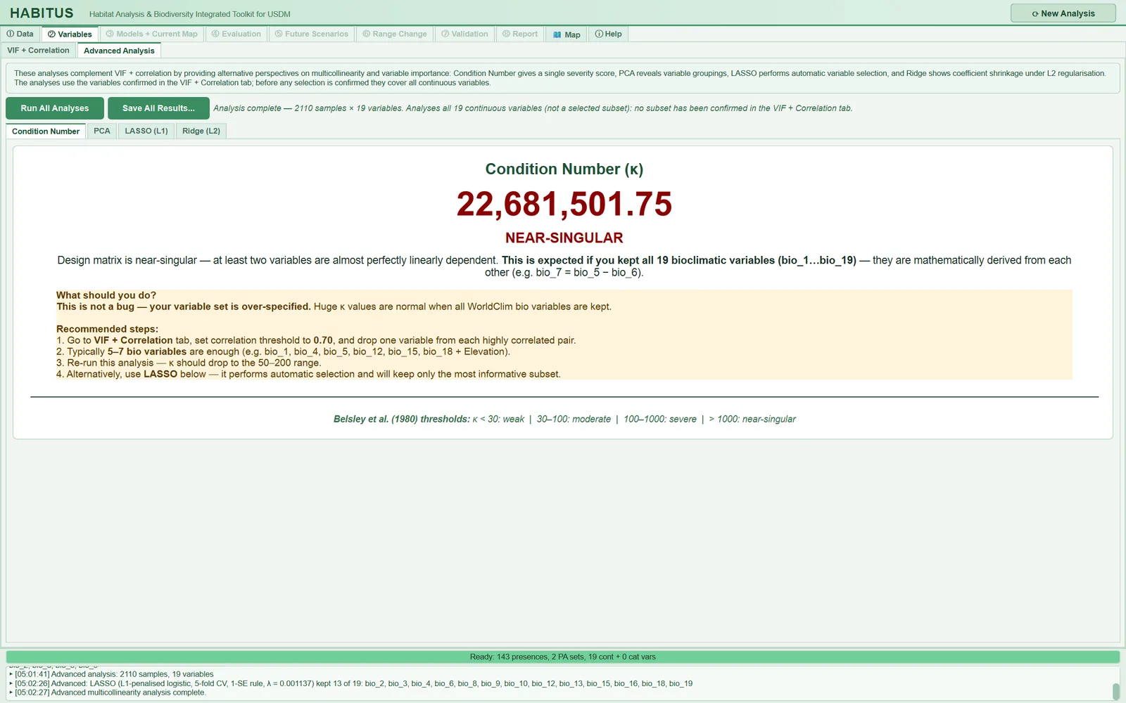
tabs/tab_vif_advanced.py:419-431). Singular values below 10^{-10} are discarded; if any are discarded, a note on near-linear dependence is added to the text. Classification: \kappa < 30LOW, 30 \le \kappa < 100MODERATE, 100 \le \kappa < 1000SEVERE, \kappa \ge 1000NEAR-SINGULAR; for each class a "What should you do?" box lists the actions to take. - When and how to set it. It has no settings. It is useful to look at it once for the full set and once after the selection: κ is expected to drop after the selection.
- Effect on results. Diagnostic only. In the example run, with 19 variables, κ = 22,681,501.75 (Figure 4.2); this is an expected value when all the mutually derived bioclimatic variables are retained.
- Caution. The thresholds on the screen are attributed to Belsley et al. (1980). Belsley's criterion consists of the condition indices and variance-decomposition proportions for each singular value; a single κ and this four-class scale are a practical summary. The suggestions in the to-do box of the NEAR-SINGULAR class ("Typically 5–7 bio variables are enough …", "κ should drop to the 50–200 range") are general guidance, not a computation specific to these data.
4.9.3 Principal components (PCA)
- What it does.
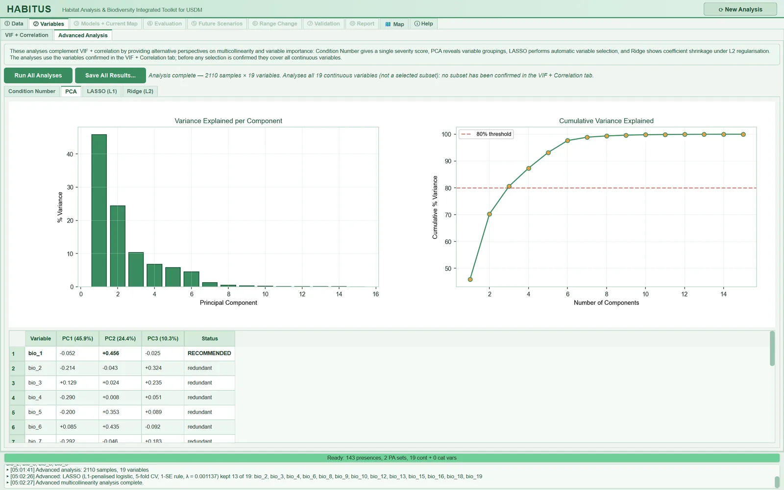
sklearn.decomposition.PCAis applied to the standardized variables (tabs/tab_vif_advanced.py:499-596). The percentage of variance explained by the first 15 components is plotted on the left, and the cumulative variance with an 80% line on the right. The table shows the loadings of the k components whose cumulative variance reaches 80% (at least 2, at most 8); the column headers give the variance share of the component ("PC1 (45.9%)"). In each component the variable with the largest absolute loading is highlighted in bold green and receivesRECOMMENDEDin theStatuscolumn; the other variables readredundant. Other cells with |\text{loading}| > 0.4 are shaded light yellow. - When and how to set it. It has no settings. It is used to see in which groups the variables cluster (for example, temperature and precipitation axes).
- Effect on results. Information only. In the example run the first three components explain 45.9%, 24.4% and 10.3% of the variance; since the cumulative 80% is exceeded at the third component, the table has three components and at most three variables receive
RECOMMENDED(in the rows visible in Figure 4.3, bio_1, with a loading of +0.456 on PC2). - Caution. The rule of "the variable with the largest loading" per component is a heuristic: if the same variable has the largest loading in two components, the number of recommended variables is less than k. The 80% limit is also conventional, a fixed value in the code (
tabs/tab_vif_advanced.py:539-540).
4.9.4 LASSO (L1) — penalized logistic regression
-
What it does. An L1-penalized logistic regression (Tibshirani 1996) is fitted to the presence (1) / pseudo-absence (0) response with standardized predictors (
tabs/tab_vif_advanced.py:43-128,638-711). Details:- Presences and absences receive equal total weight (
compute_sample_weight("balanced"); Barbet-Massin et al. 2012), so that the large number of pseudo-absences does not dominate the result. - λ is on the glmnet scale: mean weighted binomial deviance + λ × penalty; scikit-learn's
Cis taken as 1/(n\lambda). The 40-value logarithmic grid starts at the smallest λ at which no variable remains (\lambda_{\max}) and descends to \lambda_{\max}/1000. - For each λ the weighted binomial deviance is computed by stratified k-fold cross-validation; in each fold standardization uses the training part only. The number of folds is set by
CV folds, but no larger than the number of observations in the minority class and at least 2. 1-SE rule (CV): the largest λ whose deviance lies within one standard error of the minimum deviance (Hastie et al. 2009, §7.10).Minimum CV deviance: the λ with the smallest deviance.Typed value: a single fit to all data with the λ typed in the box.- Variables with an absolute coefficient larger than 10^{-8} read
SELECTED, the othersdropped. The table is sorted by absolute coefficient.
- Presences and absences receive equal total weight (
-
When and how to set it. The default
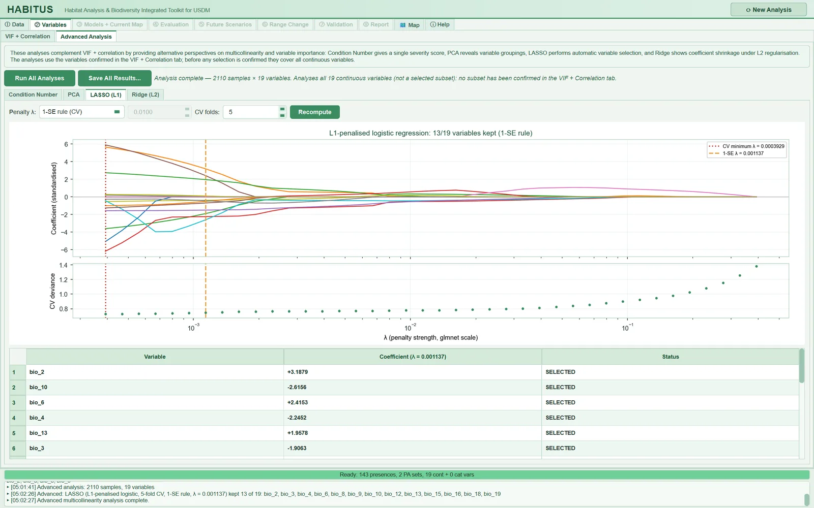
1-SE rule (CV)is the common choice for variable selection: it retains fewer and more stable variables. If predictive power is the focus,Minimum CV deviancecan be chosen. With very few presences, reducing the number of folds (3) may improve the stability of the folds. - Effect on results. Information only; it is not passed to the model settings. In the example run (19 variables, 2110 rows), with the 1-SE λ = 0.001137, 13 of the 19 variables were retained (bio_2, bio_3, bio_4, bio_6, bio_8, bio_9, bio_10, bio_12, bio_13, bio_15, bio_16, bio_18, bio_19); the λ of minimum deviance is 0.0003929 (Figure 4.4).
- Caution. LASSO picks one of a group of strongly related variables almost arbitrarily; selection among correlated variables is unstable and can change with small changes in the sample. For this reason the set retained by LASSO differs from the set of
Recommended(in the example bio_4, bio_6, bio_10, bio_12, bio_13, bio_16 were retained by LASSO but removed by stepwise VIF), and this is expected: LASSO looks at discriminatory power, stepwise VIF only at collinearity. The coefficients refer to the pooled PA sets; they are not the coefficients of the final model. In the example run the minimum deviance coincided with the smallest λ of the grid; this indicates that the grid may need to be extended to smaller λ values (see Q8).
4.9.5 Ridge (L2) — coefficient shrinkage
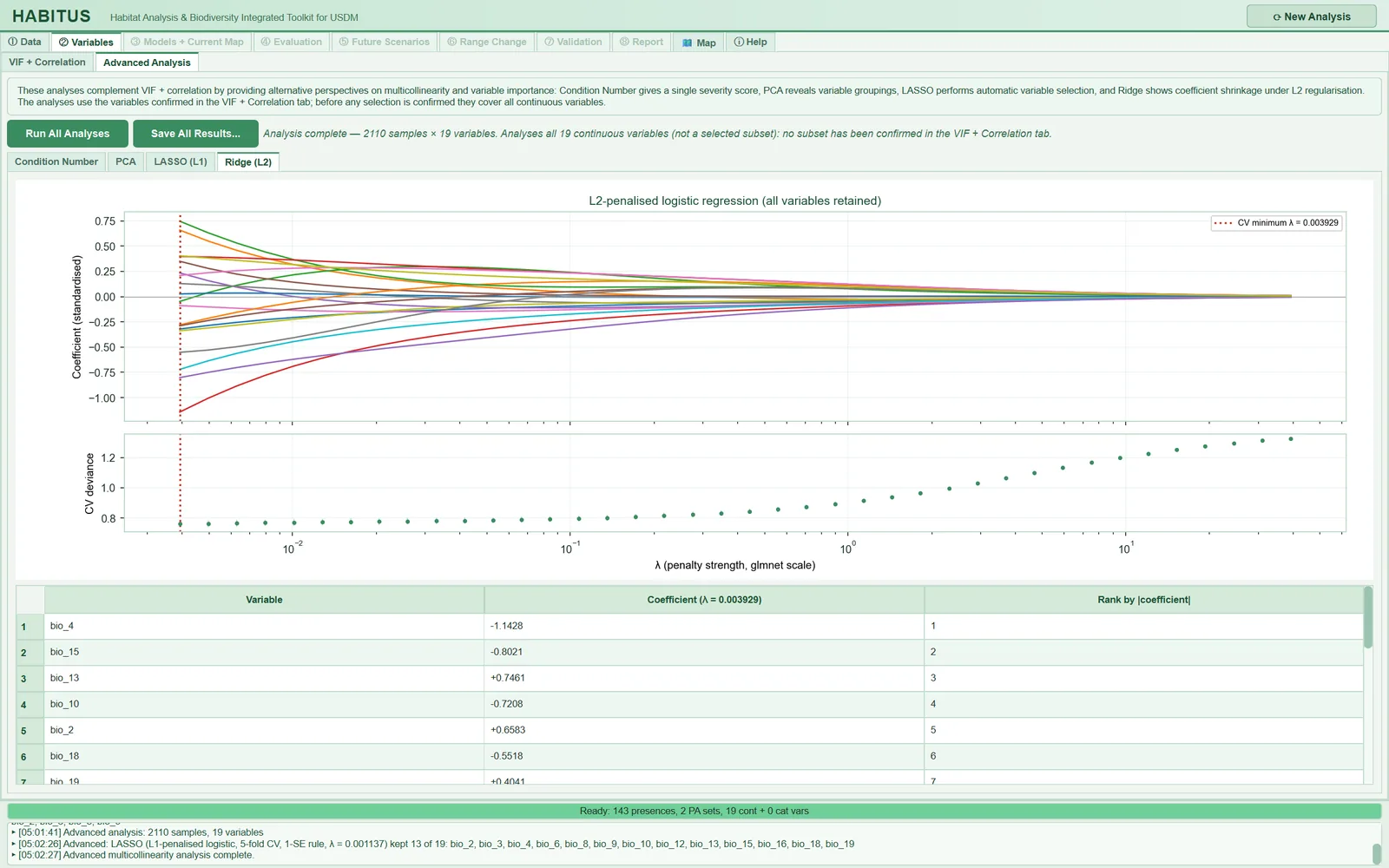
- What it does. The same set-up as LASSO, with an L2 penalty (
tabs/tab_vif_advanced.py:715-748). The grid starts at 100 \times \lambda_{\max} and descends four orders of magnitude. λ is always chosen by the minimum cross-validation deviance; it has no setting, onlyCV foldsis shared with LASSO. Ridge sets no variable to zero; the table ranks the variables by absolute standardized coefficient and gives the rank in theRank by |coefficient|column. No variable is "recommended". - When and how to set it. To see how coefficients are shared when correlated variables are kept together. Ridge coefficients are more stable than those of LASSO.
- Effect on results. Information only. In the example run λ = 0.003929; the largest absolute coefficients are bio_4 (−1.1428), bio_15 (−0.8021), bio_13 (+0.7461), bio_10 (−0.7208), bio_2 (+0.6583) (Figure 4.5).
- Caution. The
Recomputebutton recomputes LASSO only; after changingCV folds,Run All Analysesmust be pressed for Ridge to be refreshed as well. In the example run the minimum deviance of Ridge also coincided with the smallest λ of the grid.
4.9.6 Export of the advanced analysis
Save All Results... creates the advanced_analysis/ subfolder in the output folder and writes the following (tabs/tab_vif_advanced.py:760-891): condition_number.txt (κ, numbers of variables and rows, first 10 singular values), pca_variance.png, pca_loadings.csv (first k components), pca_variance.csv (variance and cumulative variance percentages of all components), lasso_coefficient_paths.png, lasso_coefficients.csv, lasso_path.csv (λ grid, CV deviance and its standard error, all coefficients), lasso_info.txt (number of records, number of folds, the two λ values, the λ used, selected variables), ridge_coefficient_paths.png, ridge_coefficients.csv, ridge_path.csv. If no output folder is defined, the warning "Set the output directory in the Data tab first." appears.
4.10 Outputs and what passes to the next step
state["var_names"]: the confirmed continuous variables, in natural name order. Used by ③ Models, ⑤ Future Scenarios (projection and novelty maps) and ⑧ Report.state["cat_selected"]/state["cat_excluded"]: the categorical selection;Noneand an empty list if there is no categorical raster.- The files in
figures/and (if requested)advanced_analysis/(§4.8, §4.9.6). - The thresholds and method of the tab are written to the report and to the "Multicollinearity" element of ODMAP.
- The records-per-predictor warning (if any) is added to the
sample_warningslist and passed to the report.
4.11 Expert questions
Q1. Does the stepwise VIF selection give the same result as usdm::vifstep?
Yes, it gives the same result on the same input. Both methods recompute the VIF of the remaining set at each step, remove the largest if it exceeds the threshold, and stop when the largest VIF is equal to or below the threshold (sdm_core.py:427-434; th = 10 in usdm). In this book they were compared on a 5000-cell WorldClim matrix: the removal order is identical for 11 variables, and the VIFs of the remaining eight variables agree to the fourteenth decimal (§4.6.2). As in usdm, VIF is computed from the R^2 of a linear regression with an intercept (sdm_core.py:275-295).
Q2. Can capping VIF at 999 change the removal order?
It can. Every variable with R^2 > 0.9999 gets a VIF of 999 (sdm_core.py:292-293); if several variables are in this state at the same step, idxmax() removes the first in natural order (sdm_core.py:430). Since usdm uses the true VIF, it removes the one that is truly the largest at that step. In the example run, bio_4 and bio_5 were removed with 999 in the first two steps. In the validation matrix this did not change the result; but in data with capped ties the final set may differ from that of usdm. The difference concerns only which of the extremely high-VIF variables goes first; if exactly the same result is required, the most obviously derived variables (such as bio_7) can be removed manually beforehand.
Q3. Why are VIF and correlation computed on the presence + pseudo-absence pool rather than on raster cells?
Because the model is trained on these points; collinearity matters in the data the model sees (tabs/tab_vif.py:349-353). As a consequence, the results depend on the extent of the accessible area and on the number of PAs (§4.3). In the VIF + Correlation pool each presence is repeated as many times as there are PA sets, whereas Advanced Analysis drops duplicates (tabs/tab_vif_advanced.py:356-363); the samples of the two sub-tabs are therefore not exactly the same. A user who wants a correlation over the whole area can apply usdm::vifstep in R directly to the rasters.
Q4. Why does Recommended not take the univariate AUC into account?
The explanation in the code: univariate discriminatory power promotes a variable that looks good in this sample thanks to its correlation with the true driver; such a variable may fail when transferred to another region or climate (sdm_core.py:323-339). For this reason both Priority_Score and Recommended are based only on collinearity, and the AUC badge is deliberately neutral in colour (tabs/tab_vif.py:471-499). Which member of a pair to drop should be decided by the ecology of the species (Dormann et al. 2013).
Q5. Why does the correlation step remove the member of a pair with the higher VIF; how does it differ from usdm::vifcor?
HABITUS first applies the VIF step, then, in the remaining set, removes from the strongest pair with |r| \ge threshold the member with the larger VIF in the current set (sdm_core.py:435-445). usdm::vifcor instead first removes variables pair by pair using the correlation threshold (from each pair, the one more strongly related to the other variables), and then looks at VIF. The final sets of the two methods may differ. With the default thresholds (VIF 10, |r| 0.80), a highly correlated pair rarely remains after the VIF step; in the example run none remained.
Q6. I changed the thresholds but Recommended gives the same suggestion. Why?
The suggestion is computed when variable_priority_ranking last ran. When the tab first opens, the pre-computation of ① Data is shown (correlation 0.70, Pearson, VIF 10; sdm_core.py:3225-3227). Changing the correlation threshold refreshes only the pairs table and the heatmap (tabs/tab_vif.py:880-884); the method and the VIF threshold refresh nothing on their own. For a new suggestion, press Run / Refresh Analysis and then Recommended.
Q7. Do LASSO and Ridge give the same results as glmnet in R?
They use the same definition (Friedman et al. 2010): binomial family, λ on the glmnet scale, equal class weights, standardized predictors, stratified k-fold cross-validation, lambda.min and lambda.1se (tabs/tab_vif_advanced.py:63-128). The program's test suite compares the coefficients at two grid points on simulated data with R glmnet: within an absolute difference of 2 \times 10^{-4} for Ridge and 3 \times 10^{-3} for LASSO, and the variables set to zero by LASSO are the same (tests/test_202_small_samples_lasso.py:81-98). The solver is liblinear and the intercept is estimated with a very small penalty (intercept_scaling=100); this is the source of small differences from glmnet. The λ grid is not the same as that of glmnet (100 values, lambda.min.ratio): HABITUS uses 40 values and descends three orders of magnitude for LASSO and four for Ridge.
Q8. What happens if the minimum cross-validation deviance falls at the end of the grid?
The program does not report this separately; lambda_min becomes the smallest value of the grid (tabs/tab_vif_advanced.py:120). In the example run this happened for LASSO (\lambda_{\min} = 0.0003929 = \lambda_{\max}/1000) and for Ridge (0.003929) (in Figures 4.4 and 4.5 the red line is at the left end). In this case the true minimum may lie at a smaller λ; the 1-SE rule, by contrast, is more reliable because the deviance curve is flat. Since these analyses are for information only, they do not affect model results; if a detailed choice of penalty is required, advanced_analysis/lasso_path.csv can be inspected or glmnet can be run with a wider grid.
Q9. Why is the condition number so large, and how does it relate to VIF?
κ is the ratio of the largest to the smallest singular value of the standardized matrix (tabs/tab_vif_advanced.py:421-431). As the smallest singular value approaches zero, κ grows; this means that at least one variable is approaching a linear combination of the others. VIF shows the same situation per variable. Because the 19 bioclimatic variables contain exact derivations such as bio_7 = bio_5 − bio_6, κ is in the millions (22,681,501.75 in the example run). A drop in κ when recomputed with the selected set shows that the selection has worked.
Q10. Can a model be built with a single variable?
No. With a single variable the ranking table is built (VIF = 1; sdm_core.py:356-368), but Confirm requires at least two continuous variables (tabs/tab_vif.py:1164-1167); Run / Refresh Analysis also asks for layers to be added in ① Data if only one variable is loaded (tabs/tab_vif.py:367-372).
Q11. Why are categorical variables not included in the collinearity check?
VIF and Pearson/Spearman correlation assume ordered numeric variables; the numeric values of categorical codes are meaningless. Categorical rasters are therefore listed separately and sparse classes (fewer than 3 presences) are flagged (tabs/tab_vif.py:583-664). The program does not measure the relationship between categorical and continuous variables (for example, a land-cover class coinciding with elevation); this is a point the user must check. Advanced Analysis does not use categorical rasters; it works only with continuous variables (tabs/tab_vif_advanced.py:343-354).
Q12. Is the selection in this tab reproducible?
VIF, correlation, PCA and the condition number involve no randomness; the same PA sets give the same result. The PA sets depend on the seed in ① Data. The cross-validation folds of LASSO and Ridge are shuffled with the run seed (formatter.random_seed) (tabs/tab_vif_advanced.py:600-604, 108). The selected variables, thresholds and method are written to the report, to ODMAP and to figures/variable_priority_ranking.csv; the removals made with Recommended are in the session log in order.
4.12 Common mistakes and pitfalls
- Changing a threshold without pressing
Run / Refresh Analysis. The suggestion stays with the old thresholds (§4.4.1). First set the thresholds, thenRun / Refresh Analysis, thenRecommended. - Treating
Recommendedas the final decision. The tooltip explicitly says "A starting point". Compare the recommended set with the ecology of the species; for example, in the example run the recommended set does not contain annual mean temperature (bio_1); bio_11 (mean temperature of the coldest quarter) has been retained instead. - Removing a recommended variable because of its full-set VIF badge. The badge shows the VIF in the presence of all variables; the VIF within the recommended set is in the
VIF_in_selectioncolumn ofvariable_priority_ranking.csv(in the example bio_11: ∞ in the full set, 2.85 in the recommended set). - Reading a red AUC in the pairs table as "drop this". The AUC colouring only compares two AUCs; a low univariate AUC does not make a variable redundant (§4.5.1).
- Changing the selection without confirming. ③ Models uses the last confirmed set. After models have been run, re-confirmation deletes everything ("Re-confirm Variable Selection").
- Assuming the suggestions of
Advanced Analysishave been applied to the list. PCA and LASSO provide information only; the ticks in the variable list do not change. - Ignoring the records-per-predictor warning. If the "Below about 10 per predictor …" warning appears, select fewer variables or use simpler algorithms in ③ Models (GLM, MaxEnt with linear/quadratic features).
4.13 References
Barbet-Massin, M., Jiguet, F., Albert, C.H., Thuiller, W., 2012. Selecting pseudo-absences for species distribution models: how, where and how many? Methods in Ecology and Evolution 3, 327–338. https://doi.org/10.1111/j.2041-210X.2011.00172.x
Belsley, D.A., Kuh, E., Welsch, R.E., 1980. Regression Diagnostics: Identifying Influential Data and Sources of Collinearity. Wiley, New York. https://doi.org/10.1002/0471725153
Dormann, C.F., Elith, J., Bacher, S., Buchmann, C., Carl, G., Carré, G., et al., 2013. Collinearity: a review of methods to deal with it and a simulation study evaluating their performance. Ecography 36, 27–46. https://doi.org/10.1111/j.1600-0587.2012.07348.x
Friedman, J., Hastie, T., Tibshirani, R., 2010. Regularization paths for generalized linear models via coordinate descent. Journal of Statistical Software 33(1), 1–22. https://doi.org/10.18637/jss.v033.i01
Hastie, T., Tibshirani, R., Friedman, J., 2009. The Elements of Statistical Learning, 2nd ed. Springer, New York. https://doi.org/10.1007/978-0-387-84858-7
Naimi, B., Hamm, N.A.S., Groen, T.A., Skidmore, A.K., Toxopeus, A.G., 2014. Where is positional uncertainty a problem for species distribution modelling? Ecography 37, 191–203. https://doi.org/10.1111/j.1600-0587.2013.00205.x
O'Brien, R.M., 2007. A caution regarding rules of thumb for variance inflation factors. Quality & Quantity 41, 673–690. https://doi.org/10.1007/s11135-006-9018-6
Tibshirani, R., 1996. Regression shrinkage and selection via the lasso. Journal of the Royal Statistical Society Series B 58, 267–288. https://doi.org/10.1111/j.2517-6161.1996.tb02080.x