10. Independent validation (⑦ Validation)
Tab: ⑦ Validation · Code: tabs/tab_validation.py (UI and computation), sdm_grid.py read_on_grid (grid alignment), tabs/tab_report.py _s9_validation (section in the report)
10.1 What this tab does
⑦ Validation compares a map produced by the model with a reference source that is independent of the model and measures map accuracy. The reference source is either a raster map (an expert-drawn range map, a published distribution map, a presence/absence layer derived from field data) or field observations whose points and reference values are given in a CSV file. The comparison is made at sample points selected on the map; the result is a confusion matrix and the metrics derived from it.
- Input: two GeoTIFFs (the reference and the map to be validated) or one GeoTIFF and one CSV. The map to be validated is usually a map written by ③ Models (for example, the ensemble binary map
EMwmean_bin). - Output: the result text (metrics, confusion matrix, per-class metrics), an optional report (
.txt,.json,.html) and a points table (.csv), and two reclassified rasters (validation/folder). The latest validation result passes to section 9 of ⑧ Report. - Lock order: the tab opens once ③ Models has finished running; at the same time the rasters in the output folder are loaded automatically into the two drop-down boxes (
tabs/tab_models.py:1848-1856).
The validation in this tab differs from the cross-validation scores in ④ Evaluation: ④ measures how well the model discriminates on its own data, using folds split from the training records; ⑦ compares the map with an external source. Neither replaces the other.
10.2 Screen layout
From top to bottom the tab consists of four numbered groups.
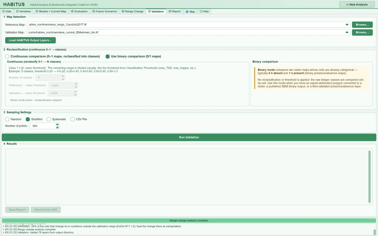
| Region | What it contains | Subsection |
|---|---|---|
1 Map Selection |
Reference Map, Validation Map, two Browse… buttons, Load HABITUS Output Layers… |
§10.3 |
2 Reclassification (continuous 0–1 → classes) |
Two mode buttons; the Continuous (reclassify 0-1 → N classes) settings on the left, the Binary comparison description on the right |
§10.4 |
3 Sampling Settings |
Random, Stratified, Systematic, CSV File; CSV path; Number of points |
§10.5 |
Run Validation |
Runs the comparison | §10.6 |
4 Results |
Result text, Save Report, Save Points CSV |
§10.6–10.8 |
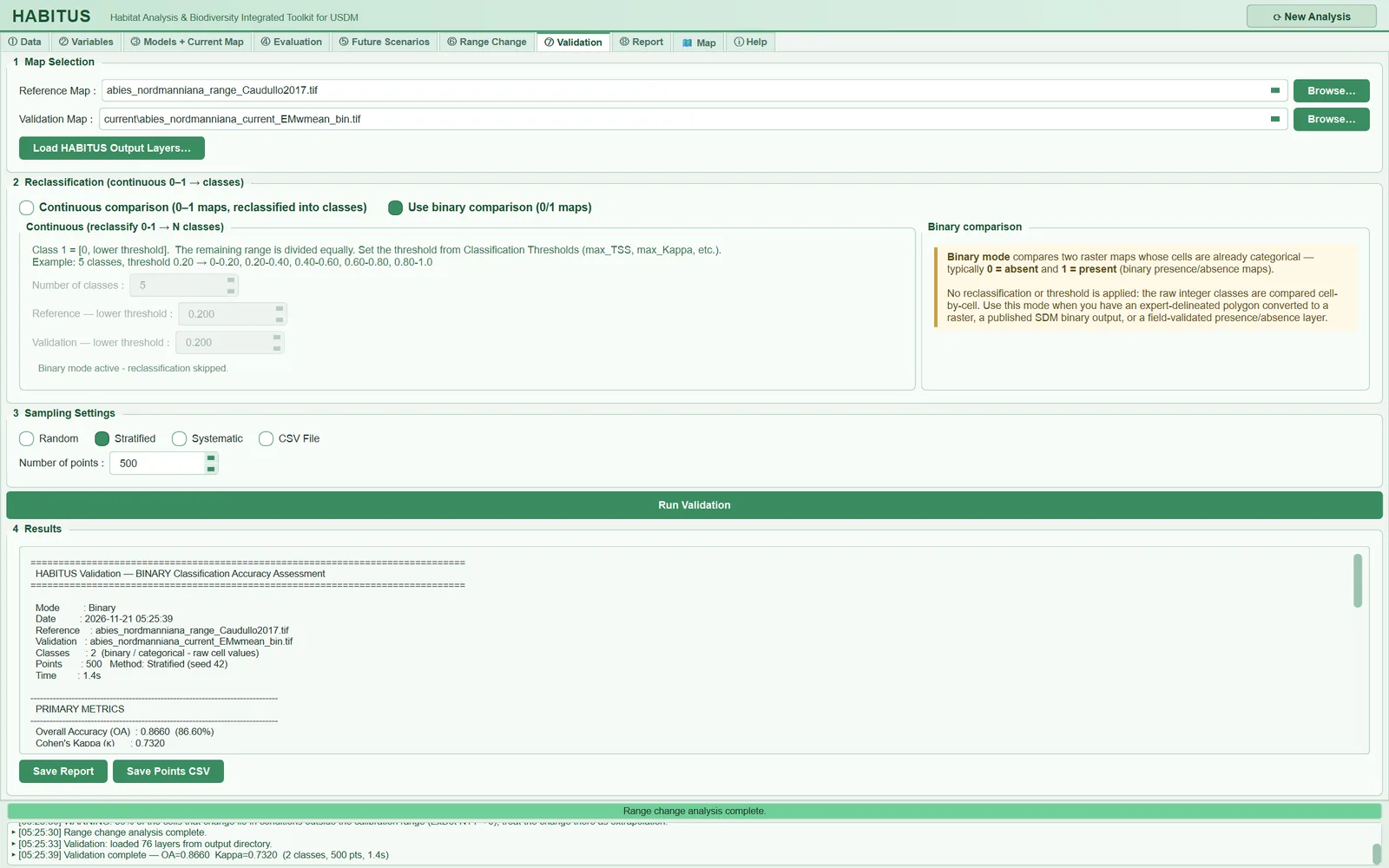
Figures 10.1 and 10.2 are taken from the example run: Abies nordmanniana; the reference map is the range map of Caudullo et al. (2017) converted to the model grid (abies_nordmanniana_range_Caudullo2017.tif), and the validated map is the ensemble binary map (current\abies_nordmanniana_current_EMwmean_bin.tif).
10.3 Map selection (1 Map Selection)
Two maps are selected: the reference map (the source taken as correct) and the map to be validated (the model's map). In the UI the latter is called Validation Map; in this chapter it is referred to as the "validated map".
| Name in the UI | What it does | Default | Range / options | Code |
|---|---|---|---|---|
Reference Map : |
Reference raster | first layer in the list | layers in the list | tabs/tab_validation.py:64-72 |
Validation Map : |
Validated raster | first layer in the list | layers in the list | tabs/tab_validation.py:74-82 |
Browse… (two) |
Selects a GeoTIFF, adds it to the corresponding list and selects it | — | *.tif, *.tiff |
tabs/tab_validation.py:341-350 |
Load HABITUS Output Layers… |
Adds all .tif files in the output folder to both lists |
automatic when the models finish | button | tabs/tab_validation.py:358-384 |
10.3.1 Loading the output layers (Load HABITUS Output Layers…)
- What it does. Scans the output folder together with its subfolders and adds every
.tif/.tifffile it finds to both lists in the same order, with a name relative to the output folder (e.g.current\abies_nordmanniana_current_EMwmean_bin.tif). It does not duplicate entries already in the list. It writes "Validation: loaded N layers from output directory." to the log; in the example run 76 layers were loaded. - When and how to set it. When ③ Models finishes, the program presses this button itself; it is pressed again to add maps written later, such as future scenarios or range change maps.
- Effect on results. A selection convenience only.
- Caution. The list contains all rasters in the output folder: probability and binary maps, individual model maps, uncertainty (
EMsd), novelty (NT1,NT2) and the accessible-area raster. Choosing the right file is up to the user. If there is no output folder, the warning "No output directory set yet. Run the analysis first." appears. The reference map is usually not in the output folder; it is added withBrowse….
10.3.2 The grids of the two maps
The comparison is made on the grid of the validated map. The reference raster is read onto this grid by position (tabs/tab_validation.py:422-455, sdm_grid.py:188-283):
- If the grids are identical, the raster is read as it is and no note is produced.
- If the cell size and coordinate system are the same and the grid is only shifted by a whole number of cells, it is copied with a shift, without interpolation.
- In every other case it is resampled with
rasterio.warp.reproject: nearest neighbour in binary mode, bilinear interpolation in continuous mode.
If an alignment was made, a note of the following form is written to the log and to the result text ("NOTE (grid)"): "Reference raster (W×H px) was not on the validation raster's grid (W×H px) and was realigned to it by position (…); N validation cell(s) not covered (x%)." If the cells not covered by the reference exceed 5% of the validated grid, an additional warning appears: "… of the validation grid lies outside the reference raster (> 5%); those cells are not compared. Check that both maps cover the same area." (tabs/tab_validation.py:447-452, sdm_grid.py:40). These notes are also passed to the "Processing notices" section of the report (state["validation_notices"]).
Caution: In continuous mode the reference map is resampled with bilinear interpolation. If the reference is a 0/1 map, intermediate values between 0 and 1 arise along the boundaries and fall into the intermediate classes. Compare a binary reference in binary mode, or prepare it on the same grid so that no resampling to the model is needed at all.
10.4 Comparison mode and reclassification (2 Reclassification)
There are two modes. The mode buttons are active in both cases; when binary mode is selected, the continuous-mode settings are greyed out and the preview line reads "Binary mode active - reclassification skipped." (tabs/tab_validation.py:191-198, 316-321).
| Name in the UI | What it does | Default | Range / options | Code |
|---|---|---|---|---|
Continuous comparison (0–1 maps, reclassified into classes) |
Reclassifies both maps into N classes and compares them | selected | mode button | tabs/tab_validation.py:100-103 |
Use binary comparison (0/1 maps) |
Rounds the cell values and compares them as they are | — | mode button | tabs/tab_validation.py:102, 599-603, 672-677 |
Number of classes : |
Number of classes in continuous mode | 5 | 2–10 | tabs/tab_validation.py:132-137 |
Reference — lower threshold : |
Upper bound of class 1 in the reference map | 0.200 | 0.000–0.990, step 0.01 | tabs/tab_validation.py:139-145 |
Validation — lower threshold : |
Upper bound of class 1 in the validated map | 0.200 | 0.000–0.990, step 0.01 | tabs/tab_validation.py:147-153 |
Ref breaks: / Val breaks: line |
Live preview of the class boundaries | — | — | tabs/tab_validation.py:155-160, 316-328 |
10.4.1 Continuous comparison (Continuous comparison)
- What it does. Both maps are divided into N classes according to their values in the 0–1 range. Boundaries: [0,\ t,\ \dots,\ 1]; class 1 is [0, t), and the remaining interval between t and 1 is divided into N-1 equal parts; the last class also includes 1 (
tabs/tab_validation.py:330-339,461-474). If t = 0, the boundaries are equally spaced between 0 and 1. Values below 0 and above 1 fall into no class and are excluded from the comparison. Class labels have the form "C1 [0.000–0.200]". - When and how to set it. When both maps are genuinely continuous (probability or suitability): for example, when comparing the probability maps of two models, or the model's probability map with the suitability map of another study. A threshold from the
Classification Thresholdstable of ④ Evaluation (such as max_TSS) can be used as the lower threshold; class 1 then means "not suitable". - Effect on results. As the number of classes increases, exact agreement becomes harder; overall accuracy and Kappa decrease. Different lower thresholds can be given for the reference and the validated map; if two models have different thresholds, this equalizes the meaning of the classes. In continuous mode, regression metrics are also computed from the raw values at the points (§10.7.3).
- Caution. If the reference is a 0/1 map, only the first and last classes are filled and the intermediate classes remain empty in the reference; the diagonal of the confusion matrix is mostly concentrated in class 1 and the metrics come out lower than in binary mode. The two modes do not measure the same thing. Use binary mode for a binary reference.
10.4.2 Binary comparison (Use binary comparison)
- What it does. The cell values of both maps are rounded to integers and compared cell by cell without applying any threshold (
np.round;tabs/tab_validation.py:601,674). The classes are taken from the data and labelled "Class 0", "Class 1". If there are two classes, the counts of true/false positives and negatives, sensitivity, specificity and TSS are added to the result text (§10.7.2). - When and how to set it. When the reference is a presence/absence map and the validated map is the model's binary map (
…_bin.tif). The description in the UI lists three typical references: a rasterized expert-drawn polygon, a published binary SDM output, a field-verified presence/absence layer. - Effect on results. In the example run (Caudullo et al. 2017 reference,
EMwmean_bin, 500 stratified points), overall accuracy is 0.866 and Kappa 0.732 (Figure 10.2). - Caution. In this mode values are rounded at 0.5; if a probability map (
…_prob.tif) is selected while binary mode is on, the map is silently split into two at the 0.5 threshold, not at the model's own threshold. A value of exactly 0.5 also goes to 0 because of NumPy's round-half-to-even rule. In binary mode always select the…_bin.tiffiles. If the labels are other than 0/1 (e.g. 1/2), TP/FP/TN/FN are assigned on the assumption that the smaller code is "absence" (tabs/tab_validation.py:908-911).
10.5 Sampling design (3 Sampling Settings)
The comparison is made not at all cells but at selected sample points. This is established practice in accuracy assessment (Congalton 1991; Olofsson et al. 2014): the result is an accuracy estimated from a sample.
| Name in the UI | What it does | Default | Range / options | Code |
|---|---|---|---|---|
Random |
Random selection without replacement from the valid cells of the classified reference | selected | method button | tabs/tab_validation.py:485-492 |
Stratified |
An equal number of cells from each class of the reference | — | method button | tabs/tab_validation.py:494-505 |
Systematic |
A regularly spaced grid over the raster | — | method button | tabs/tab_validation.py:507-520 |
CSV File |
Reference values from points in a CSV | — | method button | tabs/tab_validation.py:526-544, 622-651 |
CSV (id, x, y, reference_value): + Browse |
Path of the CSV file (visible only when CSV File is selected) |
empty | *.csv |
tabs/tab_validation.py:218-229 |
Number of points : |
Requested number of points | 500 | 30–100,000, step 50 | tabs/tab_validation.py:231-239 |
10.5.1 Random (Random)
- What it does.
Number of pointscells are selected without replacement from all valid (non-NaN) cells of the classified reference map. The random number generator is a localnumpy.random.default_rngderived from the run seed (random_seed; 42 if unknown); the same seed gives the same points, and the result text reads "Random (seed 42)" (tabs/tab_validation.py:413-420,699-701). - When and how to set it. It is the default and most easily interpreted design for estimating accuracy over the whole map: every cell has an equal probability of selection, so overall accuracy and Kappa are directly area-weighted estimates.
- Effect on results. The rare class (the species usually occupies a small part of the area) is represented by few points; the producer's and user's accuracies of that class are uncertain.
- Caution. A selected cell that is NaN in the validated map is discarded; the number of valid points may therefore be smaller than requested. The
Pointsline in the result text gives the number actually used.
10.5.2 Stratified (Stratified)
- What it does. \max(1, \lfloor n / K \rfloor) cells are selected from each class of the reference map (K is the number of classes); if a class does not have that many cells, all of them are taken (
tabs/tab_validation.py:494-505). The seed is the same as in the random design. - When and how to set it. When the producer's and user's accuracy of each class needs to be estimated with enough points, especially when the presence class is a small part of the area.
- Effect on results. Because the classes are represented by equal numbers of points, overall accuracy and Kappa are not area-weighted: each class counts with the same weight regardless of its share of the map. In the example run only 5.8% of the valid cells of the reference map are presence (4458 of 77,171 cells); the 500 stratified points, however, are half presence and half absence. From this sample, overall accuracy is 0.866 and Kappa 0.732. Over all common cells of the same two maps (77,171 cells), overall accuracy is 0.938 and Kappa 0.553 (computed for this book from the two reclassified rasters under
_calisma/validation/). Sensitivity (0.78 and 0.76) and specificity (0.95 and 0.95), on the other hand, are close in the two computations, because they are within-class proportions. - Caution. For an area-weighted estimate of overall accuracy and Kappa under a stratified design, the result of each class must be weighted by its area share in the map (Olofsson et al. 2014). The program does not perform this weighting; use the per-class metrics (producer's/user's accuracy, sensitivity, specificity, TSS) or weight the overall accuracy yourself using the
Save Points CSVoutput and the class areas. If n is not exactly divisible by K, the total number of points is smaller than n.
10.5.3 Systematic (Systematic)
- What it does. With g = \lfloor\sqrt{n}\rfloor, a regularly spaced g \times g grid is laid over the full row and column range of the raster; of the grid points, those valid in the reference are taken, stopping when n is reached (
tabs/tab_validation.py:507-520). There is no randomness; no seed is used. - When and how to set it. When regular coverage of the area is desired. It reduces the spatial autocorrelation of nearby points.
- Effect on results. Because the grid is laid over the entire rectangle of the raster, points falling in NoData areas (sea, outside the study extent) are discarded; the number of valid points is often markedly smaller than n. When 500 are requested, the grid is 22 × 22 = 484 points.
- Caution. If there is a periodic structure in the raster layout (roads, grid-shaped land use), the systematic sample may coincide with this structure.
10.5.4 CSV points (CSV File)
- What it does. Reference values are taken not from a map but from points in a CSV file. The file must be UTF-8 and its header row must contain the columns
x,y,reference_value(optionallyid); names are case-sensitive (tabs/tab_validation.py:526-544). Each point is converted to a cell with the transform of the validated raster; rows falling outside the raster, non-numeric rows or rows with a missing column are silently skipped.reference_valueis classified with the reference class boundaries (Reference — lower thresholdandNumber of classes); the validated class is read from the point's cell in the validated map (tabs/tab_validation.py:636-648). - When and how to set it. For validation with field observations, separately collected presence/absence points or point data from another study. Coordinates must be in the coordinate system of the validated raster (degrees in the example data; longitude
x, latitudey). - Effect on results.
Number of pointsis not used with this method; all valid points in the file are used. The reclassified rasters are not written in this mode. - Caution. No coordinate transformation is performed; points in a different coordinate system fall into the wrong cells or lie outside the raster and are discarded. The decimal separator must be a point (values such as "41,73" cannot be read as numbers and the row is skipped). Because
reference_valueis classified on the 0–1 scale as in continuous mode, 0/1 field data fall into the first and last classes in continuous mode; for a binary comparison with these data, see the pitfall in §10.10.
10.6 Running (Run Validation)
Run Validation runs the job in the UI thread and, while it runs, opens a small window showing the steps (tabs/tab_validation.py:550-558). The steps are written to the result box with "▸": the number of valid cells of the validated raster, its minimum/maximum/mean value and number of unique values; the class boundaries; the number of cells per class; the same for the reference; the sampling and the number of valid points. This text is then replaced by the result report (tabs/tab_validation.py:963). If no validated map is selected, the message "Please select a Validation Map." appears; if no reference is selected, "Please select a Reference Map."; if there are no common valid points, "No valid overlapping points found."
10.7 Metrics and the result text
A confusion matrix is built with scikit-learn from the (reference class, validated class) pairs at the sample points; rows are the reference, columns the validated map (tabs/tab_validation.py:749-779). The class list is the union of the classes observed on the two sides.
10.7.1 Primary metrics (PRIMARY METRICS)
| Name in the result text | Definition | Code |
|---|---|---|
Overall Accuracy (OA) |
Proportion of correctly classified points | accuracy_score, tabs/tab_validation.py:754 |
Cohen's Kappa (κ) |
Agreement corrected for chance agreement (Cohen 1960) | cohen_kappa_score, :755 |
F1-Score (Macro) / F1-Score (Weighted) |
Simple / support-weighted mean of the per-class F1 | f1_score, :756-757 |
Precision (Macro) / Recall (Macro) |
Simple mean of the per-class precision / recall | :758-759 |
Kappa Interpretation |
Verbal interpretation of Kappa (below) | :900-904 |
For all ratios, if the denominator is zero the result is taken as 0 (zero_division=0). Kappa is computed as
where p_o is the observed agreement (overall accuracy) and p_e the chance agreement expected from the class proportions of the two maps.
Kappa interpretation scale. The result text verbalizes Kappa with the following scale (tabs/tab_validation.py:900-904): \kappa < 0 "Poor"; < 0.20 "Slight"; < 0.40 "Fair"; < 0.60 "Moderate"; < 0.80 "Substantial"; otherwise "Almost Perfect". This is the scale proposed by Landis and Koch (1977). The scale is a convention proposed for inter-observer agreement; it does not provide definitive limits for map accuracy.
Caution: Kappa depends on the prevalence of the presence class (Allouche et al. 2006). The same two maps can give very different Kappa values under different sampling designs: in the example run 0.732 with the stratified sample and 0.553 over all cells (§10.5.2). Do not report Kappa alone; report sensitivity, specificity and TSS, together with the sampling design used.
10.7.2 Binary summary (BINARY SUMMARY)
In binary mode, and if there are exactly two classes, the following are added to the result text (tabs/tab_validation.py:906-922): the confusion matrix is read in the order [0, 1]; True Positive (TP), False Positive (FP), True Negative (TN), False Negative (FN); Sensitivity = TP/(TP+FN); Specificity = TN/(TN+FP); True Skill Stat TSS = sensitivity + specificity − 1 (Allouche et al. 2006). TSS is independent of prevalence; in binary validation it is a more reliable summary than Kappa.
Confusion matrix of the example run (stratified, 500 points; from the report file): of the 250 points that are absence in the reference, 238 are also absence in the model and 12 are presence; of the 250 points that are presence in the reference, 55 are absence in the model and 195 are presence. This gives sensitivity 0.780, specificity 0.952 and TSS 0.732. When equal numbers of presences and absences are sampled, Kappa and TSS take the same value; this is the reason for the equality in the example.
10.7.3 Regression metrics (continuous mode only)
In continuous mode these are computed from the raw values at the points (reference and validated, 0–1) (tabs/tab_validation.py:761-767, 923-927): R^2 (r2_score, coefficient of determination; it is not Pearson's r^2 and can be negative), RMSE, MAE, Bias = mean(validated − reference); "(Over)" is appended if it is positive and "(Under)" if negative. If the reference is a 0/1 map, these metrics measure the distance of a probability map from 0/1 and are of limited meaning.
10.7.4 Confusion matrix and per-class metrics
The result text writes three more tables (tabs/tab_validation.py:929-958):
CONFUSION MATRIX: rows are the reference classes ("Ref \ Val"), columns the validated classes.PER-CLASS METRICS: for each classPrecision,Recall,F1,Support(number of reference points in that class).PRODUCER'S & USER'S ACCURACY: producer's accuracy (the proportion of a reference class correctly shown on the map) = recall; user's accuracy (the proportion of a map class that is correct on the ground) = precision (Congalton 1991).
The beginning of the result text gives the mode, the date, the names of the reference and validated files, the number of classes, in continuous mode the two thresholds and the class boundaries, the number of points and the method (with the seed), grid notes if any, and the duration.
10.8 Export
| Name in the UI | What it does | Default | Code |
|---|---|---|---|
Save Report |
Saves the result, depending on the extension, as .txt (result text), .json (full result dictionary) or .html (summary and confusion matrix) |
validation_report_<date_time> |
tabs/tab_validation.py:970-992, 1021-1066 |
Save Points CSV |
Saves each point: id, x, y, ref_value, val_value, ref_class, val_class, match |
validation_points_<date_time>.csv |
tabs/tab_validation.py:994-1019 |
| (automatic) | In raster–raster mode, validation/Reclassify_ref_<name>.tif and validation/Reclassify_val_<ad>.tif |
— | tabs/tab_validation.py:726-730, 819-839 |
Both buttons are disabled until the first successful run. The reclassified rasters are written as float32 with NoData = −9999; if the reference was aligned, it takes the georeferencing of the validated raster. The JSON file contains the class boundaries, the confusion matrix, the class report, the seed and the grid notes; it is the most complete record for later auditing of a validation.
Section 9 of ⑧ Report uses the latest validation result in the tab (tabs/tab_report.py:2269-2320): mode, reference and validated layer, number of points, overall accuracy, Kappa, weighted F1, R², RMSE, MAE (if available), the confusion matrix and the reclassified maps. The sampling method is not included in this section; add it when writing the report.
10.9 Expert questions
Q1. Why is this validation considered "independent"; how does it differ from the scores in ④ Evaluation?
④ Evaluation is computed on cross-validation folds derived from the model's training records; the same record source and the same pseudo-absence design are used. ⑦ Validation, by contrast, compares the map with an external source (tabs/tab_validation.py:550-817). Independence depends on the nature of the reference: if the reference is a range map derived from the model's training records (for example, drawn from the same herbarium records), it cannot be considered fully independent. The program does not check the origin of the reference; the user must state it.
Q2. Do overall accuracy and Kappa obtained with stratified sampling reflect the accuracy of the map?
Not directly. Stratified takes an equal number of points from each reference class (tabs/tab_validation.py:494-505) and does not weight the results by area share. In the example run, overall accuracy and Kappa are 0.866 and 0.732 at the 500 stratified points, and 0.938 and 0.553 over all common cells (§10.5.2). For an area-weighted estimate, the stratified estimators of Olofsson et al. (2014) should be used; the program does not compute them. Within-class proportions (sensitivity, specificity, TSS) are unbiased under the stratified design as well, and reporting them is recommended.
Q3. Which metric should be reported instead of Kappa?
Kappa depends on prevalence (Allouche et al. 2006) and has been criticized in the map accuracy literature; Pontius and Millones (2011) recommend reporting quantity and allocation disagreement separately. The program does not compute quantity/allocation disagreement. In binary mode, TSS, sensitivity and specificity are in the result text (tabs/tab_validation.py:906-922); if these and the confusion matrix are reported, readers can compute the other metrics themselves. Quantity and allocation disagreement can be computed from the Save Points CSV output or from the two reclassified rasters.
Q4. What happens if the reference and the validated map have different grids?
The reference is read onto the grid of the validated map by position: an identical grid as it is, a whole-cell shift by shifting, every other case by resampling (nearest neighbour in binary mode, bilinear in continuous mode) (sdm_grid.py:188-283). The operation performed and the proportion of cells not covered are written to the result text as "NOTE (grid)"; a coverage gap exceeding 5% triggers an additional warning (tabs/tab_validation.py:436-452). If resampling involves a difference in scale (for example, a 1 km reference onto a 4.6 km model grid), nearest-neighbour selection alters the boundary cells of the reference; scale compatibility is the user's responsibility.
Q5. Over which area is sampling done; is it restricted to the accessible area?
No. Random and Stratified select from all cells that are valid in the classified reference; cells that are NaN in the validated map are then discarded (tabs/tab_validation.py:486-492, 709-722). The sampling area is thus the entire grid on which both maps have values; it is not restricted to the accessible area of ① Data. Distant, clearly unsuitable cells outside the accessible area are easily classified absences and inflate overall accuracy. To restrict the validation to the accessible area, the reference map must be set to NoData outside this area.
Q6. Is the result reproducible?
Random and Stratified use a local generator built from the run seed (random_seed; 42 if unknown) (tabs/tab_validation.py:413-420, 699); the same seed, the same maps and the same number of points give the same points. The seed is written to the result text ("Stratified (seed 42)") and to the JSON report. Systematic and CSV File involve no randomness.
Q7. Are 500 points enough; what is the uncertainty of the result?
The program does not give a confidence interval for overall accuracy or Kappa. Because the result is estimated from a single sample, it carries sampling uncertainty. Under simple random sampling the standard error of overall accuracy is approximately \sqrt{p(1-p)/n}; for p = 0.9 and n = 500 this is about 0.013. The accuracy of a rare class requires a stratified design or more points (Olofsson et al. 2014). The variability can be seen by repeating with different seeds or by increasing Number of points (up to 100,000).
Q8. How should I compare a probability map with a binary reference?
The most correct way is to use, in binary mode, the map obtained by splitting the probability map at the model's selected threshold (…_bin.tif). If a probability map is selected in binary mode, the values are rounded, i.e. a 0.5 threshold is applied (tabs/tab_validation.py:601); this is not the model's threshold. In continuous mode, on the other hand, a 0/1 reference falls only into the first and last classes and the metrics measure a mixture of two things (§10.4.1).
Q9. How should I use field presence/absence data when validating with CSV points?
With the CSV method, reference_value is always classified with the reference class boundaries (as in continuous mode) (tabs/tab_validation.py:642), whereas the validated map is read in binary mode as rounded 0/1 values. In binary mode these two codings do not match (reference 1 and N, map 0 and 1) and the result is meaningless. To compare field 0/1 data correctly, use continuous mode with Number of classes = 2 and both lower thresholds set to the same value (e.g. 0.500): the 0 and 1 of the reference then fall into classes 1 and 2 respectively, and the validated probability map is split into two classes at the same threshold. If the validated map is binary (…_bin.tif), the threshold can be any value between 0 and 1.
Q10. What are the limitations of using a range (chorology) map as the reference map? Range maps such as Caudullo et al. (2017) are expert drawings and usually show the outer limit of the species' native range; places within the limit where the species does not occur (unsuitable elevation, land use) are also counted as "presence". This increases the number of false negatives in cells that the model does not find suitable but that lie within the range. In the example run the model has more presence cells (7102) than the reference (4458); some of the places the model shows "in excess" may be climatically suitable but not reached by the species. This comparison therefore measures map agreement; it is not definitive proof of the model's biological accuracy.
Q11. Is the result passed to the report automatically, and what is missing?
Yes; section 9 of ⑧ Report uses the latest validation result (tabs/tab_report.py:2269-2320). The report does not state the sampling method or the seed; this information is in the JSON and text reports. The phrase "κ values above 0.60 are generally considered acceptable …" in the interpretive sentence of the report is a generic formula; it cites no source and does not take into account the prevalence dependence of Kappa. Before publishing the report, add the sampling design and adapt the interpretation.
10.10 Common mistakes and pitfalls
- Selecting a probability map in binary mode. Values are rounded at 0.5; the model's threshold is not used. In binary mode select
…_bin.tif. - Comparing a binary reference in continuous mode. The intermediate classes remain empty and Kappa drops artificially (§10.4.1).
- Reporting the Kappa of a stratified sample as map accuracy. This is the source of the difference between 0.732 and 0.553 in the example run (§10.5.2). State the design explicitly and report the within-class metrics.
- Wrong column name or decimal comma in the CSV. The columns must be
x,y,reference_valueand numbers must use a decimal point; non-conforming rows are skipped without warning. If no valid row remains, the message "No valid points in CSV." appears. - CSV coordinates in a different coordinate system. No transformation is performed; points fall into the wrong cell or are discarded.
- 0/1 field data from a CSV in binary mode. The codes do not match (§10.9, Q9); use continuous mode, 2 classes and equal thresholds.
- Expecting the requested number of points with
Systematic. The grid is laid over the whole rectangle; points falling in NoData are discarded. - Different extents of the reference and the validated map. Read the "NOTE (grid)" note and the coverage-gap warning; the comparison is made only in the common cells.
- Forgetting that of successive validations only the last passes to the report. Run the comparison you want to see in the report last; save the other results separately with
Save Report.
10.11 References
Allouche, O., Tsoar, A., Kadmon, R., 2006. Assessing the accuracy of species distribution models: prevalence, kappa and the true skill statistic (TSS). Journal of Applied Ecology 43, 1223–1232. https://doi.org/10.1111/j.1365-2664.2006.01214.x
Caudullo, G., Welk, E., San-Miguel-Ayanz, J., 2017. Chorological maps for the main European woody species. Data in Brief 12, 662–666. https://doi.org/10.1016/j.dib.2017.05.007
Cohen, J., 1960. A coefficient of agreement for nominal scales. Educational and Psychological Measurement 20, 37–46. https://doi.org/10.1177/001316446002000104
Congalton, R.G., 1991. A review of assessing the accuracy of classifications of remotely sensed data. Remote Sensing of Environment 37, 35–46. https://doi.org/10.1016/0034-4257(91)90048-B
Landis, J.R., Koch, G.G., 1977. The measurement of observer agreement for categorical data. Biometrics 33, 159–174. https://doi.org/10.2307/2529310
Olofsson, P., Foody, G.M., Herold, M., Stehman, S.V., Woodcock, C.E., Wulder, M.A., 2014. Good practices for estimating area and assessing accuracy of land change. Remote Sensing of Environment 148, 42–57. https://doi.org/10.1016/j.rse.2014.02.015
Pontius, R.G., Millones, M., 2011. Death to Kappa: birth of quantity disagreement and allocation disagreement for accuracy assessment. International Journal of Remote Sensing 32, 4407–4429. https://doi.org/10.1080/01431161.2011.552923