8. Future scenarios (⑤ Future Scenarios)
Tab: ⑤ Future Scenarios · Code: tabs/tab_projection.py (UI), sdm_core.py Projector (computation), sdm_novelty.py (ExDet, MESS), sdm_grid.py (grid alignment), sdm_mask.py (clipping to the study boundary)
8.1 What this tab does
The ⑤ Future Scenarios tab applies the models built in ③ Models to another stack of environmental layers; this is called projection (transfer). The most common use is to apply a model built with current climate to the future-period layers of a climate model (GCM, general circulation model). The same tab is also used to transfer the model to another region or to a past period: the program only expects "continuous rasters with the same names and in the same order as the variables used in training".
The tab is unlocked when ③ Models has finished (tabs/tab_models.py:1849). The map for current climate has already been produced in ③ (the current\ subfolder of the output folder, tabs/tab_models.py:1719); ⑤ produces the future counterpart of this map.
- Input: one continuous raster for each model variable (scenario layers), the selection of algorithms to project, and the optional MESS/MoD, MESS mask and clamping options.
- Computation: each full-data model (each algorithm × pseudo-absence set) is applied to the new layers; within-algorithm mean and spread maps, ensemble maps, binary (0/1) maps and ExDet novelty surfaces are written (
sdm_core.py:7733-8156). - Output: GeoTIFF files and the
<species>_<scenario>_projection_options.jsonrecord in the scenario subfolder; the list of files in theCompleted Projectionstable; the maps in the map viewer on the right. - Tab unlocked: when the job finishes, ⑥ Range Change is unlocked (
tabs/tab_projection.py:672).
8.2 Screen layout
The tab has two panes: the settings on the left, the map viewer and the ▶ Run Projection button on the right (tabs/tab_projection.py:98, ui_style.two_pane).
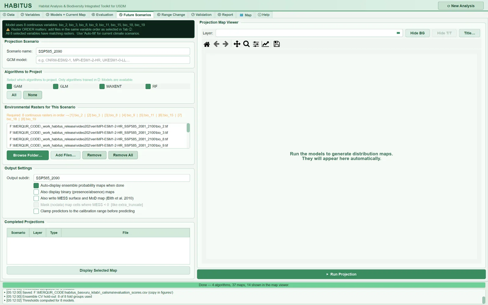
The regions of the left pane, from top to bottom, are:
| Region | Name in the UI | Described in |
|---|---|---|
| Information banner | (untitled, dark green box) | §8.3 |
| Scenario name and GCM | Projection Scenario |
§8.4 |
| Algorithm selection | Algorithms to Project |
§8.5 |
| Raster list | Environmental Rasters for This Scenario |
§8.6 |
| Output and method options | Output Settings |
§8.7, §8.8 |
| Completed outputs | Completed Projections |
§8.11 |
| Map | Projection Map Viewer (right pane) |
§8.12 |
8.3 Information banner
The dark box at the top of the tab is rewritten every time the tab is shown (tabs/tab_projection.py:308-345). It gives three pieces of information:
- The continuous variables used by the model (
Model uses 8 continuous variables: bio_2, bio_3, …). - The order warning:
⚠ Raster ORDER matters: add files in the same variable order as selected in Tab ②. - Whether the training rasters match the variables (
All 8 selected variables have matching rasters.orWarning: only k/n variables matched …). If there are categorical variables, a line is added saying that they are not carried into the future and that the current layer is reused.
The orange line immediately below (Required: 8 continuous rasters in order → [1] bio_2 | [2] bio_3 | …) shows the order of the files to be added, numbered (tabs/tab_projection.py:340-343).
Note: There is no button in this tab corresponding to the phrase
Use 'Auto-fill' for current climate scenarios.that appears in the banner. The current climate map is produced automatically in ③ Models; a user who wants to re-project current climate with other settings (e.g. with MESS on) selects the folder of the training rasters withBrowse Folder…(§8.6.2).
8.4 Scenario name and GCM (Projection Scenario)
| Name in the UI | What it does | Default | Range / options | Code |
|---|---|---|---|---|
Scenario name: |
Name of the projection; enters the file names, the subfolder, the report and the list in ⑥ | 2050_SSP245 |
free text; current if empty |
tabs/tab_projection.py:115, :505 |
GCM model: |
Climate model name to be written in the map title | empty | free text | tabs/tab_projection.py:119, :31-44 |
8.4.1 Scenario name
- What it does. The scenario name (
proj_name) enters the name of every output file:<species>_<scenario>_<layer>_prob.tif(sdm_core.py:7895). IfOutput subdir:is empty, it is also the name of the output folder (tabs/tab_projection.py:544). The name is kept as a key in the session state (state["projections"][name]); the ⑥ Range Change lists, the novelty table in the report and the multi-species batch run work with this key (tabs/tab_projection.py:580,:636). - When and how to set it. The name should state both the period and the scenario:
SSP585_2090,SSP245_2050_MPI. If more than one GCM is used, include the GCM in the name as well; otherwise the outputs of two GCMs are written to the same folder and the same file names. - Effect on results. It has no effect on the computation; it determines the organisation of files and records.
- Caution. If an SSP5-8.5 2090 layer is projected without changing the default text
2050_SSP245, the files are written with the wrong name; the program does not check the name against the content. Running a second time with the same name overwrites the same files and duplicates the rows in the table. Naming itcurrentoverwrites the current maps produced by ③ (the samecurrent\folder) and thecurrentrecord in the session.
8.4.2 GCM name
- What it does. It is only added to the map title in the viewer (
Future Distribution · MPI-ESM1-2-HR · SSP585_2090 · …,tabs/tab_projection.py:690-691). It does not enter the file names, the report or ODMAP. - Caution. If the GCM information is to appear in the report and files, it must be written into the scenario name.
8.5 Algorithms to project (Algorithms to Project)
| Name in the UI | What it does | Default | Range / options | Code |
|---|---|---|---|---|
algorithm boxes (e.g. GAM, GLM, MAXENT, RF) |
Which algorithms' models are projected | all checked | algorithms trained in ③ | tabs/tab_projection.py:288-306 |
All / None |
Checks all / unchecks all | — | — | tabs/tab_projection.py:142-145 |
- What it does. Each time the tab is opened, the boxes are built as a grid of four per row from the models trained in ③ (
modeler.fitted_models). The full-data models of the selected algorithms ("Full", the model refitted with all data; one for each pseudo-absence set) are projected (sdm_core.py:7850-7855). IfAlso project the cross-validation models (more replicates, slower)was checked in ③, the cross-validation models are projected as well (tabs/tab_models.py:1537,:1546). - When and how to set it. If the current map and the future map are to be compared (⑥ Range Change), the two maps must be produced with the same set of algorithms; therefore leaving all algorithms used in ③ checked is the default and recommended choice. If an algorithm is known to behave poorly in transfer (e.g. a GAM that jumps outside the range), leaving it out can be done as a sensitivity test.
- Effect on results. An unselected algorithm does not enter the ensemble map; the ensemble weights are computed only over the projected models (
sdm_core.py:8028-8035). In the example run, with four algorithms selected, 8 models (4 algorithms × 2 pseudo-absence sets) were projected and 37 rasters were written. - Caution. If no box is checked, the message
Select at least one algorithm to project.appears. If none of the selected algorithms passes the ensemble criterion in ③ (minimum score), no ensemble map is written and the warningWARNING: No full-data model reached the minimum …appears in the log (sdm_core.py:8036-8054).
8.6 Raster list and the order rule (Environmental Rasters for This Scenario)
| Name in the UI | What it does | Default | Range / options | Code |
|---|---|---|---|---|
| raster list | Continuous layers of the scenario, in variable order | empty | multiple selection | tabs/tab_projection.py:159-162 |
Browse Folder… |
Matches the rasters in a folder to the variable names and fills the list | — | .tif .tiff .asc .img .nc .vrt |
tabs/tab_projection.py:166-170, :382-449 |
Add Files… |
Appends the selected files to the end of the list | — | same extensions | tabs/tab_projection.py:172, :451-457 |
Remove |
Deletes the selected rows | — | — | tabs/tab_projection.py:174, :459-461 |
Remove All |
Deletes the list and all projection results, locks ⑥ | — | asks for confirmation | tabs/tab_projection.py:177-180, :463-489 |
8.6.1 The order rule
- What it does. The program matches continuous rasters by position: the i-th file in the list is read as the i-th continuous variable of the model (
sdm_core.py:7335,:7407-7412). There is a single exception: if the names of the files in the list (in cleaned form, e.g.bio_ (12)→bio_12) form exactly the same set as the model variables, the files are matched by name even if the order differs (sdm_core.py:7375-7379). This prevents alphabetically sorted lists such asbio_11, bio_15, bio_18, bio_19, bio_2, …from swapping two layers. - When and how to set it. Storing the future layers with the same file names as the training layers (
bio_2.tif,bio_3.tif…) is the safest course; then name matching takes effect and an order error becomes impossible. If the file names differ (such aswc2.1_2.5m_bioc_MPI_ssp585_2081-2100_02.tif), the list must be built exactly in the order of the orange line. - Effect on results. An order error does not stop the program: if two variables are swapped, the model takes, for example, precipitation seasonality for temperature and the map becomes meaningless. The only trace revealing this is an unusually high ExDet NT1 proportion (§8.9).
- Caution. The number of files must equal the number of continuous variables of the model; otherwise the message
Raster count mismatch!appears and the projection does not start (tabs/tab_projection.py:525-534,sdm_core.py:7360-7366). Categorical variables (land cover, soil class) are not added to this list: the program takes them from the current categorical rasters loaded in ① Data and assumes them to be the same in the future (sdm_core.py:7474-7483,:7414-7442). That is, land cover is assumed not to change.
8.6.2 Adding from a folder (Browse Folder…)
- What it does. The names of the raster files in the selected folder are converted to lower case and spaces, parentheses, hyphens and dots are reduced to underscores; for each model variable, the program searches in turn for (1) an exact name match, (2) a file name that starts with the variable name, (3) the variable name occurring within the file name (
tabs/tab_projection.py:399-436). The matches are written to the list in variable order. - When and how to set it. With a layout in which each scenario is kept in a separate folder and with the same names as in training, the correct list is built with a single click (in the example run
MPI-ESM1-2-HR_SSP585_2081_2100\bio_2.tif …). - Effect on results. With a correct match, it gives the same result as a manually built list.
- Caution. The "prefix" and "contains" rules are loose: for the variable
bio_1the exact name is searched first; if it is not found, the first file starting withbio_1, such asbio_10.tiforbio_11.tif, may be taken. Unmatched variables are listed in theUnmatched Variablesdialog and the user is asked to add them withAdd Files…. After the list has been built, check it visually against the orange line.
8.6.3 Adding and removing files
Add Files… appends the selected files to the end of the list; keeping the order is up to the user. Remove deletes only rows in the list. Remove All, however, after asking for confirmation, clears the list, resets all projection and range change results in the session, empties the maps and tables of both tabs and locks ⑥ Range Change again (tabs/tab_projection.py:475-489). Files on disk are not deleted.
8.7 Output and display settings (Output Settings)
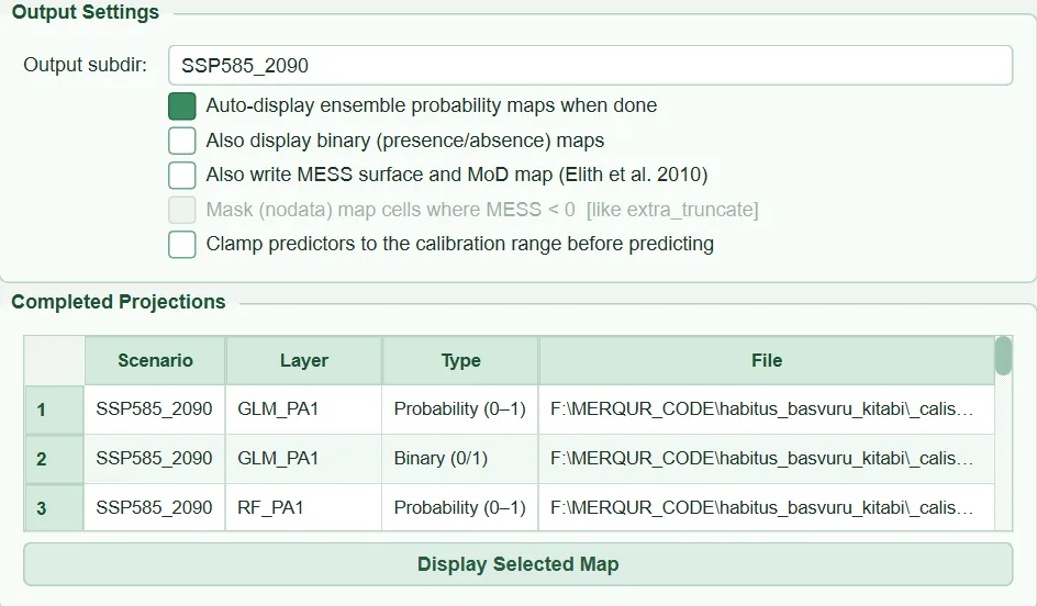
| Name in the UI | What it does | Default | Range / options | Code |
|---|---|---|---|---|
Output subdir: |
Subfolder to which the scenario files are written | empty (scenario name is used) | free text | tabs/tab_projection.py:197-198, :543-545 |
Auto-display ensemble probability maps when done |
Loads the probability maps into the viewer when the job finishes | on | on / off | tabs/tab_projection.py:199-201, :669-670 |
Also display binary (presence/absence) maps |
Also loads the binary maps | off | on / off | tabs/tab_projection.py:202-203, :683-684 |
Also write MESS surface and MoD map (Elith et al. 2010) |
Also writes the MESS and MoD rasters | off | on / off | tabs/tab_projection.py:204-214 |
Mask (nodata) map cells where MESS < 0 [like extra_truncate] |
Sets cells with MESS < 0 to nodata in the maps | off (disabled while MESS is off) | on / off | tabs/tab_projection.py:215-224 |
Clamp predictors to the calibration range before predicting |
Clips the predictors to the training range before prediction | off | on / off | tabs/tab_projection.py:225-233 |
8.7.1 Output subfolder
- What it does. Files are written under
<output folder>\<Output subdir>; if the field is empty, the scenario name is used (tabs/tab_projection.py:544-545). - When and how to set it. In most cases it is left empty. A different subfolder can be given to compare two runs of the same scenario with different settings (e.g. clamping on/off); however, because the file names are generated from the scenario name, ⑥ and the report distinguish the two runs only if the scenario names also differ.
- Caution. The report (⑧) looks for the PNGs of the future maps in these subfolders (§11.5.7); saving the scenario PNGs here determines the layout of the report.
8.7.2 Display options
While Auto-display … is on, the viewer is cleared when the job finishes and all probability maps whose names end in _prob are loaded: not only the ensemble but also the single models and the algorithm means (14 maps in the example run, tabs/tab_projection.py:675-705). If Also display binary … is on, the _bin maps are added as well. These two options do not change any file; they only fill the viewer's Layer: list.
8.8 Transfer safety options: MESS, MESS mask, clamping
A model produces a value between 0 and 1 even under environmental conditions it never saw in training; this value appears as "certain" as the others. The narrower the environmental range of the calibration area, the more often this happens in transfer (Owens et al. 2013). HABITUS handles this problem at three levels: ExDet is computed automatically in every projection (§8.9); MESS is an optional additional diagnostic; the MESS mask and clamping change the map itself.
All three use the same calibration reference set: the rows on which the models were actually built, i.e. the union of the presence and absence points in all pseudo-absence sets (sdm_core.py:7142-7171, :4929-4952). Categorical variables do not enter the reference.
8.8.1 MESS and MoD (Also write MESS surface and MoD map)
- What it does. Following the definition of Elith et al. (2010), a similarity value is computed for each cell and each variable. With F the percentage of reference points whose value of variable j is less than or equal to p, \min_j the smallest value and \max_j the largest (
sdm_novelty.py:377-449):
MESS is the smallest of the s_j; MoD (most dissimilar variable) is the index of the variable giving this smallest value. The files written are <species>_<scenario>_MESS.tif (float32) and <species>_<scenario>_MoD.tif (int16; the variable names are stored in the raster labels as CLASS_i) (sdm_core.py:7263-7281).
- When and how to set it. MESS is turned on in studies that require comparison with the outputs of the MaxEnt software and dismo/flexsdm, or where a reviewer asks for a "MESS map". In terms of method, ExDet NT1 already gives the same information (§8.9).
- Effect on results. It does not change the suitability maps. The line MESS: x% of projected cells have MESS < 0 … is written to the log (sdm_core.py:7286-7289). Because the same reference set and the same minimum/maximum values are used, the cells with MESS < 0 are the same as the cells with ExDet NT1 < 0 (if a value is exactly equal to the maximum, both give 0): in the example run, the NT1 < 0 proportion for SSP585_2090 is 55.4%; had MESS been turned on, the same proportion would have been reported for MESS < 0. The only difference is a variable that is constant in training: NT1 ignores it, whereas MESS gives −100 to every cell that differs from the constant value (sdm_novelty.py:216-225, :436-437).
- Caution. MESS is univariate: it cannot see cells where the combination is novel while all variables are individually within range; for these, ExDet NT2 is consulted. The tooltip text says this too: MESS cannot see novel combinations of in-range values; ExDet NT2 can.
8.8.2 MESS < 0 mask (Mask (nodata) map cells where MESS < 0)
- What it does. After all outputs have been written, cells with MESS < 0 are set to nodata (−9999) in the probability, binary, algorithm mean, algorithm spread (
_sd) and ensemble spread (EMsd,EMcv,EMrange) maps (sdm_core.py:7293-7325,:8112-8123). The ExDet and MESS/MoD rasters are not masked. It is the counterpart of theextra_truncatefunction in flexsdm (Velazco et al. 2022). The box is not enabled unless the MESS box is checked (tabs/tab_projection.py:224). - When and how to set it. Turned on when the map will be used directly for a decision (conservation priority, area computation) and extrapolated cells should not be interpreted at all. In a scientific report, the unmasked map and the NT1 map are usually given side by side and the masked computation is added as a sensitivity analysis.
- Effect on results. The effect is large. Because MESS < 0 and NT1 < 0 are the same cells, in the example run the mask would have set 55.4% of the cells of the SSP585_2090 map to nodata. ⑥ Range Change counts only cells that are valid in both maps (
sdm_core.py:8292); a masked future map does not count the masked cells as "lost" or "gained", it removes them from the computation entirely. Thus the current area, too, is computed only from current presence cells lying outside the mask. - Caution. If MESS cannot be computed, no masking is done and
WARNING: MESS truncation was requested but MESS could not be computed; the maps of <scenario> were NOT truncated.is written to the log (sdm_core.py:8114-8119). Whether masking was done can be read from themess_truncateandmess_truncated_filesfields of the_projection_options.jsonfile.
8.8.3 Clamping (Clamp predictors to the calibration range before predicting)
- What it does. Before prediction, each continuous variable in the projection is clipped to the minimum and maximum values of the reference set (
np.cliplogic;sdm_core.py:7808-7814,:4929-4960). Single models, algorithm means and the ensemble predict with these clipped values. ExDet and MESS, however, are computed with the unclipped raw values; that is, the novelty maps continue to show the actual extrapolation. - When and how to set it. Algorithms that fit flexible response curves (quadratic terms of GLM, GAM curves, MaxEnt hinge/product features) can rise and fall outside the range and produce unrealistic values; tree-based methods (RF, GBM, BRT), on the other hand, already stay constant at the last value outside the range. If the NT1 proportion in the future layers is high (55.4% in the example run), making two projections, with and without clamping, and reporting the difference is good practice. This is the logic of the "clamping" option in the MaxEnt software and of the
do.clamping/clamping.maskapproach in biomod2. - Effect on results. In out-of-range cells, suitability is fixed at the suitability of the value at the edge of the range. In tree-based methods the effect is small; in GLM/GAM/MaxEnt it can be marked in extrapolated cells. The gain/loss proportions in ⑥ are affected by these cells.
- Caution. Clamping does not remove extrapolation, it only holds the response constant; the assumption is made that "the condition at the edge of the range continues outside the range". The clamping setting in ③ Models (
settings.models.clamp) governs the current map; the box in ⑤ is chosen separately for each scenario and written to the_projection_options.jsonfile. For comparability, use the same choice for the current and future maps.
8.9 ExDet novelty surfaces (always written)
There is no box for this in the UI: Projector runs ExDet in every projection (write_novelty=True, sdm_core.py:7088, :7937-7943). The method is the ExDet of Mesgaran et al. (2014) and it distinguishes two kinds of novelty.
NT1 (univariate range novelty). With \min_j the smallest and \max_j the largest value of variable j in the reference set, for cell i (sdm_novelty.py:202-228):
Within the range NT1 = 0, outside it is negative; the larger the absolute value, the further outside the range the cell lies.
NT2 (combinational novelty). Only in cells with NT1 = 0, the squared Mahalanobis distance D^2 is computed with the mean and covariance of the reference set and divided by the largest D^2 in the reference set: NT2_i = D^2_i / \max(D^2_{ref}) (sdm_novelty.py:249-290). NT2 > 1 marks a cell where each variable on its own is within range but the combination was never seen in training.
MIC (most influential covariate). For NT1, the variable giving the most negative UD_{ij}; for NT2, the variable whose removal reduces D^2 the most (Mesgaran et al. 2014, eq. 7; sdm_novelty.py:231-235, :292-317).
Files written: <species>_<scenario>_NT1.tif, _NT2.tif, _MIC_NT1.tif, _MIC_NT2.tif (MIC values are variable indices; the names are in the raster labels as CLASS_i; sdm_core.py:7206-7233). A plain-text summary is written to the log (sdm_novelty.py:640-692). The SSP585_2090 summary of the example run:
| Measure | current | SSP585_2090 |
|---|---|---|
| NT1 < 0 (out of range) | 23.4% | 55.4% |
| NT2 > 1 (novel combination) | 0.0% | 0.3% |
| Similar according to both tests | 76.6% | 44.3% |
| Most influential variable, range novelty | bio_3 (43%), bio_15 (24%), bio_2 (13%) | bio_9 (58%), bio_3 (17%), bio_8 (10%) |
When the NT1 proportion exceeds 25%, the warning More than a quarter of the projection is outside the calibration range. Treat the suitability surface in those areas as an extrapolation, not a prediction. is added to the log (sdm_novelty.py:686-690).
Caution: The reference set consists of the presence and pseudo-absence points; this is why even in the current map 23.4% of the cells come out with NT1 < 0: because the training points are selected from within the accessible area (in the example, 200 km around the records), the distant corners of the study area are outside the range even today. This is not an error but a finding that says that this part of the map is also an extrapolation.
Note: If the condition number of the calibration covariance matrix exceeds 10^{12} (variables that are near copies of each other), NT2 is not computed; the reason is written to the log and the report:
NT2 was not computed: the calibration covariance matrix is numerically singular …(sdm_novelty.py:62,:257-265). NT1 is written in this case too.
8.10 Grid alignment, clipping to the study boundary and strip-wise projection
These three operations require no settings from the user, but they directly affect the result and the meaning of the warnings the program gives needs to be understood.
8.10.1 Grid alignment
- What it does. Each scenario layer is fitted by position onto the training grid (transform, number of rows and columns, coordinate system) (
sdm_grid.py:188-280,sdm_core.py:7486-7498): - if the grid is the same, the file is read as it is;
- if the cell size is the same and the offset is a whole number of cells, the values are shifted without interpolation (
cell-shift); - in every other case the layer is resampled with
rasterio.warp.reproject: bilinear for continuous layers, nearest neighbour for categorical layers.
Training cells not covered by the layer become NaN and are counted; a cell with NaN is excluded from the projection (cells in which all variables are finite are predicted, sdm_core.py:7799-7807).
- When and how to set it. Downloaded GCM sets may be one cell wider than the training layers or cut differently; alignment brings them together safely. It is best to prepare the future layers at the same resolution and extent as the training layers; then no resampling is done.
- Effect on results. Shifting and identity do not change the values; resampling (especially from a different resolution) smooths the values.
- Caution. For every aligned layer, a line is written to the log and to the Processing Notices section of the report, for example WARNING grid alignment: bio_2: 468x222 px grid realigned to 466x220 reference by position (cell-shift), offset -1 col / -1 row, 0 reference cell(s) not covered (0.0%). If a layer does not cover more than 5% of the training grid, the additional warning … % of the reference grid is outside this layer's extent (> 5%); those cells are NaN and are left out of the projection. Check that the layer covers the study area. appears (sdm_grid.py:40, :304-328). The summary is stored in the grid_alignment field of the _projection_options.json file; in the example run n_realigned: 0 (all eight layers on the training grid).
8.10.2 Clipping to the study boundary
- What it does. If a study boundary was given in ① Data, the future rasters are also clipped to the same boundary and placed on the grid of the clipped training rasters (
tabs/tab_projection.py:589-613,sdm_mask.py:304-418). The clipped copies are written under<output folder>\masked_inputs\<scenario>\with their original file names, so that name matching is not broken. If all files in the list are already the (clipped) files used in training, clipping is skipped (tabs/tab_projection.py:590-592). - Effect on results. The current and future maps cover the same area cell by cell; ⑥ compares like with like.
- Caution. During clipping, layers with a different cell size are moved onto the training grid by nearest neighbour and
Resampled to the training grid (nearest neighbour, another cell size): …is written to the log (tabs/tab_projection.py:610-613,sdm_mask.py:273-301). Without a boundary, in the same situation, continuous layers are resampled bilinearly (§8.10.1). If future layers of a different resolution are to be used, bringing them to the training resolution beforehand removes this difference. If the boundary does not overlap the layer, or a layer has no data at all within the boundary, the job stops with an explicit message (sdm_mask.py:369-403).
8.10.3 Strip-wise projection (large rasters)
- What it does. If the training grid exceeds 4 million cells (default strip size 2 million cells; the grid is split if it is larger than twice this), the raster is projected in row strips and the strips are merged into the same files (
sdm_core.py:7514-7527,:7566-7682). Because each cell is predicted on its own, the result is the same as a single-piece computation; the ExDet and MESS summaries are obtained by summing the counts from the strips (sdm_novelty.py:452-637). - When and how to set it. There is no user setting. The strip size can be changed with the
HABITUS_PROJECTION_TILE_CELLSenvironment variable (0 = no splitting). A user who gets an out-of-memory error can reduce this value. - Effect on results. The values are the same; the run time increases slightly and memory use decreases.
Large raster (… cells): projecting in k strips of up to n rows to keep memory in check.is written to the log. - Caution. Intermediate strip files are written to a temporary folder named
.habitus_strips_*in the output folder and deleted when the job finishes; the output disk needs as much free space as the final maps. Layers that are not on the training grid are first aligned once and written to this folder.
8.11 Outputs and the Completed Projections table
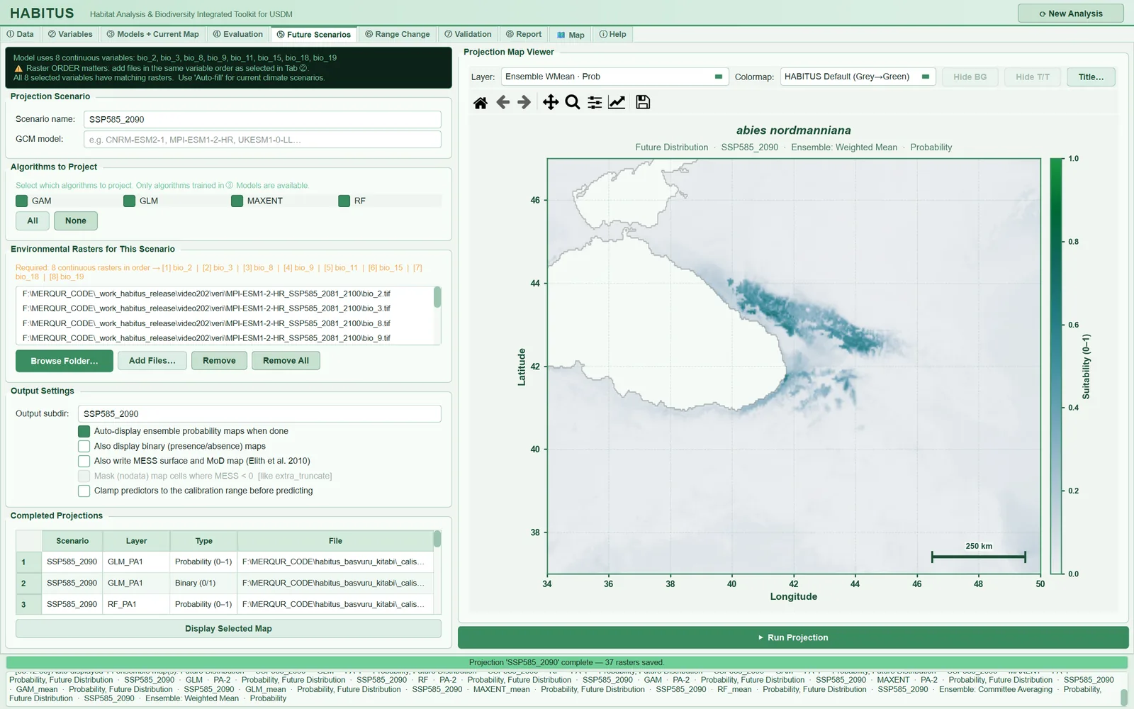
In the example run, 37 rasters and one JSON record were written to the SSP585_2090\ folder:
File (<species>_<scenario>_…) |
Content | Code |
|---|---|---|
<ALG>_PA<k>_prob.tif, _bin.tif |
Probability and binary map of a single model (threshold: the threshold found for that model in ③) | sdm_core.py:7895-7916 |
<ALG>_mean_prob.tif, _mean_bin.tif, _sd.tif |
Mean, binary and standard deviation over the replicates of the algorithm (if the two-level ensemble is on in ③) | sdm_core.py:7964-8023 |
EMwmean_prob.tif, EMca_prob.tif and _bin |
Weighted-mean and committee-averaging ensemble maps | sdm_core.py:8055-8103 |
EMsd.tif (and, if selected, EMcv, EMrange) |
Spread among the ensemble members; not thresholded | sdm_core.py:8057-8068 |
NT1, NT2, MIC_NT1, MIC_NT2 |
ExDet surfaces | sdm_core.py:7227-7233 |
MESS, MoD |
Only if MESS was selected | sdm_core.py:7279-7281 |
_projection_options.json |
clamp, mess, mess_truncate, number of masked files, MESS < 0 proportion, grid alignment summary | sdm_core.py:8126-8143 |
All probability maps are float32, nodata −9999 and in the 0–1 range; the map is not stretched to its own range, so that thresholds and scenarios remain comparable (sdm_core.py:7884-7889). If the source raster has geographic coordinates (or no coordinate system), EPSG:4326 is assigned to the output; for a projected source the original system is kept (sdm_core.py:7830-7837). The ensemble binary threshold is 0.5 (majority vote) for committee averaging, and for the weighted mean it is the mean of the members' thresholds with the same weights (sdm_core.py:6423-6446).
| Name in the UI | What it does | Default | Range / options | Code |
|---|---|---|---|---|
Completed Projections table |
One row for each output file: Scenario, Layer, Type, File |
empty | row selection | tabs/tab_projection.py:243-257, :644-662 |
Display Selected Map |
Loads the map of the selected rows into the viewer | — | — | tabs/tab_projection.py:259-262, :709-733 |
The Type column shows Probability (0–1) for probability maps and Binary (0/1) for binary maps; for novelty and spread files the last part of the key (e.g. NT1, sd) appears.
Caution:
Display Selected Mapdraws every row that does not sayProbabilitywith the binary colour scale. To inspect NT1, NT2, MESS or_sdmaps, opening these files in GIS software or in the 🗺 Map tab gives a more accurate display.
8.12 Map viewer (Projection Map Viewer)
The viewer in the right pane (RasterMapWidget, tabs/tab_projection.py:265-272) is the same as the current map viewer in ③: the Layer: list shows the loaded layers by their short names (Ensemble WMean · Prob, GLM · PA1 · Bin), Colormap: selects the colour scale of the probability map, Hide BG hides the background country borders, Title… edits the title; the disk icon in the toolbar saves the map at journal column width. The title is built from the scenario, GCM, ensemble method and map type (tabs/tab_projection.py:31-44). All controls of the viewer and the publication output are described in Chapter 12.
Tip: Save the PNG of the future map into the scenario subfolder (e.g.
SSP585_2090\) so that it enters the report. The save dialog opens by default in the root of the output folder; a PNG saved to the root enters the "6. Current Distribution" section of the report (§11.5.6).
8.13 Outputs and what passes to the next step
state["projections"][<scenario>]: a key → file path dictionary. TheCurrent proj. key/Future proj. keylists in ⑥ Range Change are built from it (only layers with_binin their name).state["novelty"][<scenario>]: ExDet summary; the novelty table in the report (§11.5.8) and the extrapolation share in ⑥ use it and theNT1.tiffile.state["grid_alignment"],state["projection_settings"]: processing notes in the report and ODMAP.run_log: the raster list, algorithms and options of the scenario; the multi-species batch run in ⑧ repeats this record (tabs/tab_projection.py:580-584).
8.14 Expert questions
Q1. Are future rasters matched by name or by order? How is an order error prevented?
Answer: The basic rule is position: the i-th file is the i-th continuous variable (sdm_core.py:7335, :7407). However, if the (cleaned) file names form the same set as the model variables, the program corrects the order according to the names (sdm_core.py:7375-7379). If the file names differ, no correction is possible. The most robust course is to store the future layers with the same names as in training and to use Browse Folder…. In biomod2, BIOMOD_Projection matches the new environment by layer names; in HABITUS, name matching takes effect only when the names match exactly.
Q2. What is the reference set of ExDet? Why are MaxEnt's background points not included?
Answer: The reference is the union of the presence + absence rows in all pseudo-absence sets (sdm_core.py:7142-7171). Mesgaran et al. (2014) recommend choosing the reference according to the modelling approach; in a presence-background model, this is the environment the model has seen. MaxEnt, however, is additionally built with 10,000 background points (maxent_background, sdm_core.py:3916, :4596-4598), and these points are not added to the reference. Points outside the accessible area are absent from both sets; however, because MaxEnt's background may cover a wider environmental range, ExDet may be somewhat pessimistic (showing more novelty) from MaxEnt's point of view. This effect has not been measured.
Q3. Do MESS and ExDet NT1 give different results?
Answer: With the same reference, the set of out-of-range cells is the same: MESS < 0 occurs only if a value is smaller than the minimum or larger than the maximum (sdm_novelty.py:431-435); NT1 < 0 is exactly this as well (sdm_novelty.py:221-225). The values differ (MESS is the smallest similarity on a percentage scale, NT1 the sum of range-normalised distances), the sign is the same. MESS additionally gives cells within the range a similarity between 0 and 100; NT1 is 0 there. The difference appears for a variable that is constant in training (§8.8.1).
Q4. Why is the NT2 threshold 1? Mahalanobis distance or its square?
Answer: The code computes D^2 (the square) and divides it by the largest D^2 in the reference set (sdm_novelty.py:271-290). A cell whose ratio exceeds 1 is "further away" than even the most extreme point in the reference set; this is the criterion of Mesgaran et al. Taking the square or the root does not change the threshold of 1 (monotonic transformation). The inverse of the covariance matrix is obtained with pinv; if the condition number exceeds 10^{12}, NT2 is not computed (sdm_novelty.py:257-269).
Q5. Does clamping change the ExDet and MESS results?
Answer: No. Clipping is applied only to the prediction matrix (X_valid); ExDet and MESS are computed from the raw X_flat (sdm_core.py:7808-7814, :7937-7955). Thus even with clamping on, the novelty maps show the actual extrapolation. The clipping range for clamping is also the minimum/maximum value of the reference set (sdm_core.py:4929-4952).
Q6. Which models are projected; where are the cross-validation models?
Answer: By default, for each algorithm and each pseudo-absence set, the "Full" model refitted with all data is projected; this corresponds to the allData behaviour of biomod2 (Thuiller et al. 2009) (sdm_core.py:7846-7855). If Also project the cross-validation models is selected in ③, the fold models are projected as well, and the algorithm mean and spread rest on more replicates; the file names carry the run label, such as PA1_RUN1 (sdm_core.py:7874). This choice is made in ③, not in ⑤, and is kept there for consistency with the current map (tabs/tab_models.py:1538-1546).
Q7. Where does the threshold of the future binary map come from? Is it recomputed from the future data?
Answer: No. For each model, the threshold found from cross-validation in ③ (tss_thresholds, default method max TSS) is used unchanged (sdm_core.py:7908); the ensemble threshold is the weighted mean of the members' thresholds for the weighted mean, and 0.5 for committee averaging (sdm_core.py:6423-6446). Since there are no observations in the future, re-estimating the threshold would be impossible anyway. Because the probability maps are not stretched, this threshold is meaningful on the same scale in both periods (sdm_core.py:7884-7889).
Q8. How are categorical variables (land cover) handled in the future?
Answer: Categorical rasters are not added to the future list; the current categorical rasters loaded in ① Data and used in the model are read again (sdm_core.py:7474-7483). That is, categorical variables are assumed not to change. If a future land cover scenario is to be used, the program does not support this; the variable must be converted to a continuous layer (e.g. forest proportion) and modelled as continuous.
Q9. What happens if the future layers have a different resolution?
Answer: Without a study boundary, continuous layers are resampled to the training grid bilinearly and categorical layers by nearest neighbour (sdm_grid.py:263-280); with a boundary, nearest neighbour is used during clipping (sdm_mask.py:273-301). In both cases a warning is written to the log and the report. Resampling a coarse GCM layer onto a fine grid produces no information; it only equalises the number of cells. It is recommended that training and projection be prepared at the same resolution (after downscaling if necessary).
Q10. Why does the range change differ when the MESS < 0 mask is on?
Answer: The masked cells become nodata in the future map; ⑥ counts only cells that are valid in both maps (sdm_core.py:8292). These cells become neither loss nor gain but "excluded from the computation"; both the current and the future area shrink. In the example run this means removing 55.4% of the cells. Reporting the two results, with the mask on and off, together shows how much the result depends on extrapolation. The Accessible area without extrapolation option in ⑥ answers the same question without changing the map (§9.6).
Q11. How is an average over several GCMs made instead of a single GCM?
Answer: The program does not produce an ensemble across GCMs or a scenario uncertainty surface; the ODMAP record says so too (odmap.py, "Uncertainty through scenarios"). Each GCM is projected under a separate scenario name; mean and spread maps are computed outside the program (e.g. R terra::app). The difference between GCMs is often larger than the difference between algorithms; in a study done with a single GCM this limitation should be stated.
Q12. Is the projection reproducible?
Answer: There is no random component in the projection: the same models and the same rasters give the same map. The models themselves are determined by the seed in ① Data. The options used are written to the _projection_options.json file (sdm_core.py:8126-8143), and the raster list and algorithms to the run_log in the session; the raster paths do not enter the report or the run record, so the source of the GCM files used must be stated separately in the methods text.
8.15 Common mistakes and pitfalls
- Not changing the default scenario name. If SSP5-8.5 layers are projected under the name
2050_SSP245, all files and the report carry the wrong name. - Mixing up the order. When name matching does not take effect (file names differ), an order error passes without a message. Its symptoms are an unusually high NT1 proportion and an unexpected variable in the
Most influential predictor for range noveltyline. - Adding a categorical variable to the list. The message
Raster count mismatch!appears; categorical layers are reused automatically. - Running a second GCM under the same name. The files are overwritten in the same folder. Use a separate name for each GCM.
- Assuming that
Remove Allonly clears the list. This button resets all projection and range change results in the session and locks ⑥. - Using the MESS mask without saying so. An area computation made with a masked map leaves out the extrapolated cells; if this is not stated in the methods, the reader misinterprets the loss proportion.
- Different clamping in the current and future maps. The clamping choice in ③ and in ⑤ is made separately; if they differ, part of the range change comes from the difference in method.
- Ignoring NT1. In the example run, more than half of the future cells are out of range; the suitability in these cells is not a prediction but an extrapolation.
8.16 References
Elith, J., Kearney, M., Phillips, S., 2010. The art of modelling range-shifting species. Methods in Ecology and Evolution 1, 330–342. https://doi.org/10.1111/j.2041-210X.2010.00036.x
Mesgaran, M.B., Cousens, R.D., Webber, B.L., 2014. Here be dragons: a tool for quantifying novelty due to covariate range and correlation change when projecting species distribution models. Diversity and Distributions 20, 1147–1159. https://doi.org/10.1111/ddi.12209
Owens, H.L., Campbell, L.P., Dornak, L.L., Saupe, E.E., Barve, N., Soberón, J., Ingenloff, K., Lira-Noriega, A., Hensz, C.M., Myers, C.E., Peterson, A.T., 2013. Constraints on interpretation of ecological niche models by limited environmental ranges on calibration areas. Ecological Modelling 263, 10–18. https://doi.org/10.1016/j.ecolmodel.2013.04.011
Thuiller, W., Lafourcade, B., Engler, R., Araújo, M.B., 2009. BIOMOD – a platform for ensemble forecasting of species distributions. Ecography 32, 369–373. https://doi.org/10.1111/j.1600-0587.2008.05742.x
Velazco, S.J.E., Rose, M.B., de Andrade, A.F.A., Minoli, I., Franklin, J., 2022. flexsdm: An R package for supporting a comprehensive and flexible species distribution modelling workflow. Methods in Ecology and Evolution 13, 1661–1669. https://doi.org/10.1111/2041-210X.13874