7. Evaluation (④ Evaluation)
Tab: ④ Evaluation · Code: tabs/tab_evaluation.py (UI); sdm_core.py evaluate_all, boyce_ecospat, compute_calibration, cv_roc_curves, cv_omission_pr_calibration, cv_boyce_curves, cv_threshold_performance, compute_response_curves, evaluation_scores_table (computation)
7.1 What this tab does
④ Evaluation shows the performance of the models built in ③ Models in charts and tables. It does not build new models or re-split the data: all curves and scores are produced from the out-of-fold (CV hold-out) predictions saved during the ③ Models run (sdm_core.py:5547-5556, 6826-7037). Only two things are computed from the full-data (Full) models: the response curves (§7.7) and the map thresholds in the Classification Thresholds table (§7.9).
- Input: the modeller (
modeler) and ensemble (ensemble) objects of ③ Models, the PA sets, the output folder. - Output: seven sub-tabs on screen; PNG figures (300 dpi) in the
figures/folder,evaluation_scores.csv,evaluation_omission_pr_calibration.csv,classification_thresholds.csv(§7.11). - Locking: unlocked when the ③ Models run finishes (
tabs/tab_models.py:1848). When the tab is first shown, all charts are computed once, accompanied by a progress window; switching tabs does not recompute for the same run (tabs/tab_evaluation.py:1344-1371).
7.2 Screen layout
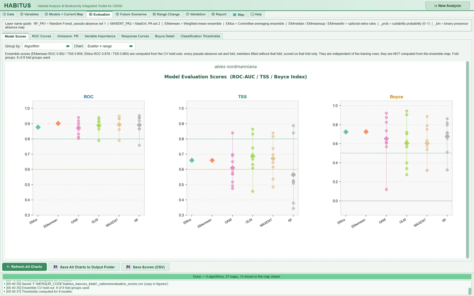
Figure 7.1. ④ Evaluation tab with the Model Scores sub-tab open: the layer name guide at the top, seven sub-tabs in the middle, ROC, TSS and Boyce panels with Group by = Algorithm and Chart = Scatter + range (including the EMca and EMwmean ensemble rows), and the Refresh All Charts, Save All Charts to Output Folder and Save Scores (CSV) buttons at the bottom.
| Area | Content | In this chapter |
|---|---|---|
| Top strip | Layer name guide: meaning of the layer names (RF_PA1, EMwmean, _prob, _bin …) |
§7.2 |
Model Scores |
ROC, TSS, Boyce distributions | §7.3 |
ROC Curves |
Out-of-fold ROC curves | §7.4 |
Omission & PR |
Omission, precision-recall, calibration | §7.5 |
Variable Importance |
Permutation importance | §7.6 |
Response Curves |
Response curves (marginal / partial / ice) | §7.7 |
Boyce Detail |
Boyce P/E curves per fold | §7.8 |
Classification Thresholds |
Thresholds of eleven threshold rules and their out-of-fold performance | §7.9 |
| Bottom buttons | ↻ Refresh All Charts, 💾 Save All Charts to Output Folder, 💾 Save Scores (CSV) |
§7.10 |
In the sub-tab strip, the name of the third sub-tab appears on screen as Omission PR; in the code its name is Omission & PR (tabs/tab_evaluation.py:201). This chapter uses the name in the code.
Multi-row figures (scores, ROC, omission, response, Boyce) sit in their own scroll area; if the figure continues below, the hint ▼ Scroll down for more of this figure appears (tabs/tab_evaluation.py:69-101).
7.3 Model scores (Model Scores)
This sub-tab (Figure 7.1) plots the ROC, TSS and Boyce columns of the evaluation_scores.csv table in three panels (tabs/tab_evaluation.py:229-353). The table itself contains every metric; the metrics are defined in §7.3.2.
| Name in the UI | What it does | Default | Options | Code |
|---|---|---|---|---|
Group by: |
Column used to group the points | Algorithm |
Algorithm / PA Set / CV Run |
tabs/tab_evaluation.py:233-235 |
Chart: |
Chart type | Scatter + range |
Scatter + range / Box plot / Bar mean±SD |
tabs/tab_evaluation.py:237-239 |
| Ensemble note | Writes the hold-out scores and fold groups of the ensemble rows | — | — | tabs/tab_evaluation.py:261-281 |
7.3.1 Chart and grouping
What it does. Scatter + range draws each row as a point, the group's minimum–maximum range as a line and the mean as a diamond; Box plot draws a box plot; Bar mean±SD draws a mean and standard deviation bar (tabs/tab_evaluation.py:315-331). The ROC and TSS panels have dashed lines at 0.8 (green) and 0.6 (orange), the Boyce panel lines at 0.5 and 0. If there are more than six groups, the labels are written vertically.
When and how to set it. Algorithm compares algorithms; PA Set shows the difference between pseudo-absence sets (the effect of background sampling); CV Run shows the difference between folds (whether some folds are systematically difficult).
Effect on results. Changes only the view; the table and files do not change.
Caution. The chart uses all rows of the table: CV runs, Full rows carrying the CV mean, and ensemble rows (PA Set = Ensemble). Because Full rows are copies of the mean, in Algorithm grouping one extra mean point per PA set is added to an algorithm's distribution; when reading the spread, rely on the Score_source = cv_fold rows in evaluation_scores.csv. The lower axis limits are 0.3 for ROC and TSS and −0.15 for Boyce (tabs/tab_evaluation.py:314); values below these are not visible in the panel.
7.3.2 Metrics in the score table
Each row is computed by evaluate_all from a model's predictions (sdm_core.py:1122-1257). Threshold-dependent metrics are computed at the threshold found with the threshold rule and threshold source selected in ③ Models (train_cv by default) (Chapter 6, §6.5). TP, FN, FP, TN are the cells of the confusion matrix; if a denominator is zero, the metric becomes NaN, not 0 (sdm_core.py:693-719).
| Column | Definition | Threshold-dependent | Code |
|---|---|---|---|
ROC |
Area under the ROC curve (AUC) | no | sdm_core.py:951-959 |
TSS |
Sensitivity + specificity − 1 (Allouche et al. 2006) | yes | sdm_core.py:671-679 |
Boyce |
Continuous Boyce index (ecospat or legacy definition) | no | sdm_core.py:475-664 |
Threshold |
Binary threshold used | — | sdm_core.py:1242 |
Prevalence, N_pres, N_abs |
Proportion and numbers of presences in the evaluation set | no | sdm_core.py:1249-1252 |
PredPresFrac |
Proportion of rows above the threshold | yes | sdm_core.py:1235-1236 |
Brier |
\overline{(p-y)^2}; smaller is better | no | sdm_core.py:998 |
CalSlope |
Slope of the logistic regression of y on \mathrm{logit}(p); 1 good calibration, <1 overconfident (Pearce and Ferrier 2000) | no | sdm_core.py:1000-1013 |
Sensitivity, Specificity |
TP/(TP+FN), TN/(TN+FP) | yes | sdm_core.py:709-710 |
Kappa |
Cohen's kappa (Fielding and Bell 1997) | yes | sdm_core.py:711-712 |
MCC |
Matthews correlation coefficient | yes | sdm_core.py:713-714 |
Jaccard, Sorensen, FPB |
TP/(TP+FP+FN); 2TP/(2TP+FP+FN); 2 × Jaccard (Li and Guo 2013) | yes | sdm_core.py:715-719 |
OR_MTP, OR_10p |
Proportion of test presences below the lowest / 10th percentile prediction of the training presences | depends on reference threshold | sdm_core.py:1095-1099 |
AUC_train, dAUC |
AUC on the training data; AUC_train − ROC (overfitting gap) |
no | sdm_core.py:1074-1084 |
OR_MTP_degenerate, OR_10p_degenerate |
1 if the omission threshold is equal to or below the smallest prediction (omission is 0 by construction) | — | sdm_core.py:1100-1114 |
Threshold_source, OR_reference, Boyce_formula |
Source of the threshold, the omission reference and the Boyce definition | — | sdm_core.py:5877-5879 |
Score_source |
cv_fold, cv_mean, random_split, cv_holdout |
— | sdm_core.py:1038-1053 |
Score_source values: cv_fold is the score of a CV run on its own held-out fold; cv_mean is the CV mean carried over to the full-data model; random_split is the random-split score of a full-data model for which no CV score was produced (optimistic); cv_holdout is an ensemble row (Chapter 6, §6.6.7).
Note:
compute_calibrationalso computes the calibration intercept (CalIntercept) and the maximum and expected calibration errors (MCE,ECE) (sdm_core.py:981-1033); these three values are not written toevaluation_scores.csv.
A row from the example run (GLM, PA1, RUN1): ROC 0.941, TSS 0.865, Boyce 0.399, threshold 0.177, prevalence 0.148 (43 presences, 248 absences), sensitivity 0.953, specificity 0.911, calibration slope 1.28, AUC_train 0.900 (dAUC = −0.041). In the RUN2 fold of the same algorithm, ROC is 0.790 and TSS 0.457; the difference between folds is larger than the difference between algorithms.
7.4 ROC curves (ROC Curves)
Figure 7.2. ROC Curves sub-tab: a separate panel for each algorithm and ensemble rule; thin lines are individual folds, the thick line is the mean curve, the shading is the ±1 SD band.
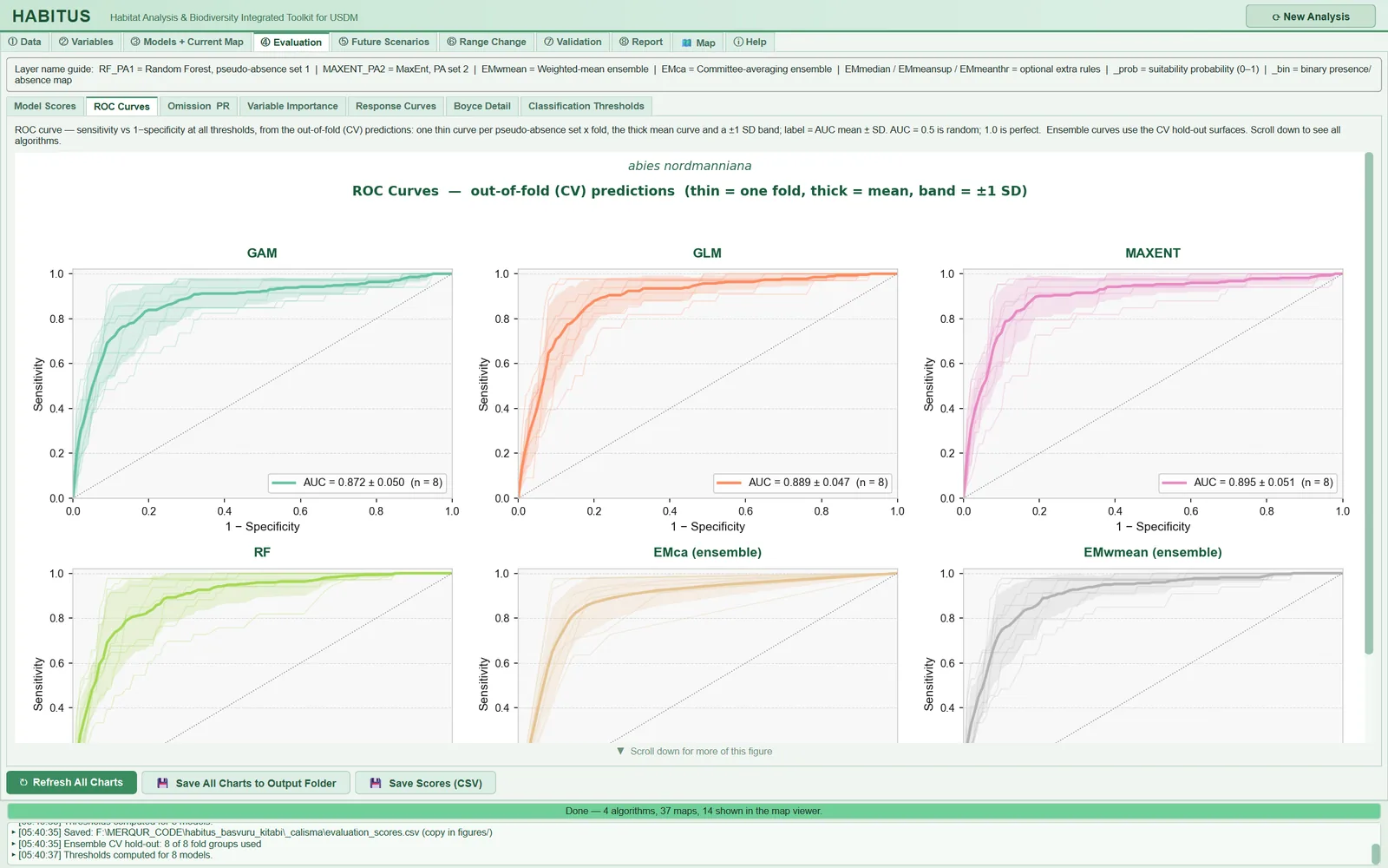
What it does. For each algorithm, one ROC curve is drawn from the out-of-fold predictions of each PA set × fold group; the curves are interpolated onto a common 101-point false positive rate grid, and the mean curve and ±1 SD band are computed; the legend has the form AUC = mean ± SD (n = number of fold groups) (cv_roc_curves, sdm_core.py:6826-6891; tabs/tab_evaluation.py:372-435). Ensemble rules (EMwmean (ensemble) …) are drawn from the ensemble's hold-out surfaces (Chapter 6, §6.6.7). There are no settings.
Effect on results. Screen and evaluation_roc_curves.png; the scores do not change. In the example run, AUC over eight fold groups: GAM 0.872 ± 0.050, GLM 0.889 ± 0.047, MaxEnt 0.895 ± 0.051.
Caution. A single-class hold-out is skipped; an algorithm with no out-of-fold predictions at all is listed below the figure with the note Not shown: … (sdm_core.py:6872-6876; tabs/tab_evaluation.py:427-429). Because the absence class consists of pseudo-absences, AUC is the ability to "discriminate presence points from the background"; it is not a measure of performance against true absences.
7.5 Omission, precision-recall and calibration (Omission & PR)
Figure 7.3. Omission & PR sub-tab: omission rate, precision-recall and calibration panels in one row for each algorithm, thin curves per fold and the mean.
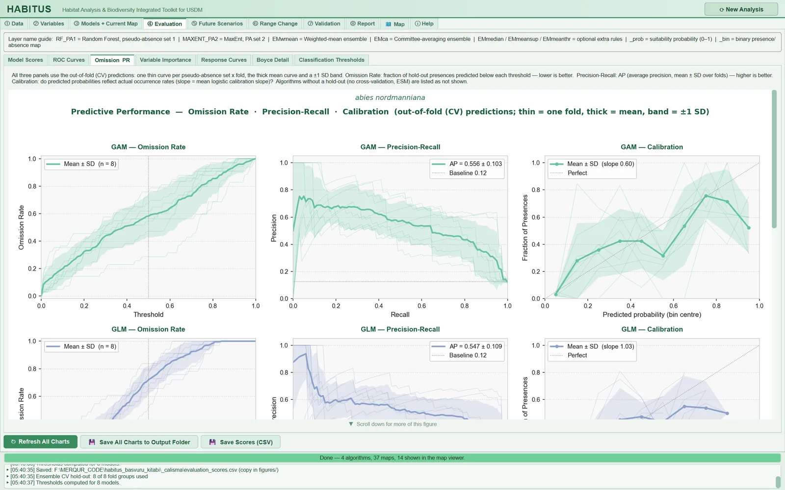
What it does. For each algorithm, three panels are drawn from the out-of-fold predictions (cv_omission_pr_calibration, sdm_core.py:6926-6995; tabs/tab_evaluation.py:459-571):
- Omission Rate: at 101 thresholds between 0 and 1, the proportion of hold-out presences whose prediction falls below the threshold. Lower is better; there is a dashed vertical line at 0.5.
- Precision-Recall: the precision-recall curve, interpolated onto a common recall grid; the legend is average precision (AP) ± SD. The grey horizontal line is the baseline precision (mean of the fold prevalences).
- Calibration: predictions are divided into 10 equal-width bins; the proportion of presences is computed in each bin (bins with fewer than 3 rows are left empty); the legend is the mean calibration slope of the folds. The diagonal indicates perfect calibration.
Effect on results. Screen, evaluation_omission_pr_calibration.png, and figures/evaluation_omission_pr_calibration.csv, which contains for each algorithm the mean omission at the 0.5 threshold, AP, baseline precision and mean calibration slope (tabs/tab_evaluation.py:573-597).
In the example run, AP is 0.556 ± 0.103 (baseline 0.12) with a mean calibration slope of 0.60 for GAM, and AP 0.547 ± 0.109 with a slope of 1.03 for GLM: the two models discriminate similarly, but GAM's probabilities are overconfident.
Caution. With pseudo-absence data, precision and calibration cannot be interpreted as absolute values: the "absence" class is background, and the probability scale depends on the PA:presence ratio (7:1 in the example run, baseline precision about 0.12). These panels are for comparing algorithms and folds with each other. Because the hold-out sets are small (32–43 presences per fold in the example run), the ±1 SD band is not a confidence interval.
7.6 Variable importance (Variable Importance)
Figure 7.4. Variable Importance sub-tab: bars of mean permutation importance per algorithm for each variable; the legend box is to the right of the chart.
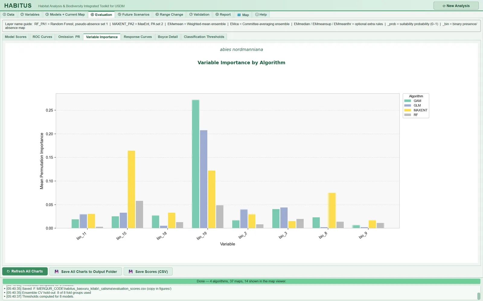
What it does. The permutation importance computed on the test fold in each CV run in ③ Models (the drop in AUC when a predictor is shuffled) is averaged for each algorithm × variable over all folds and PA sets and plotted in a grouped bar chart (tabs/tab_evaluation.py:607-647; computation: sdm_core.py:5562-5636). There are no settings; the number of repetitions is the Variable importance reps: field in ③ Models (Chapter 6, §6.4.7).
When and how to set it. Importance values are on the same scale across algorithms (AUC drop); nevertheless, tree-based and linear models may rank importance differently, so look for consistency across algorithms for a common ranking.
Effect on results. Screen and evaluation_variable_importance.png. In the example run, the most important variable in GAM and GLM is bio_19 (AUC drop of about 0.27 and 0.21, respectively), and in MaxEnt bio_15 (about 0.16); in RF no variable exceeds 0.06.
Caution. Correlated predictors share importance: when one is shuffled, the other continues to carry the information, and both may appear unimportant. Importance can be negative (shuffling increased AUC by chance). If Variable importance reps: = 0, the chart stays empty. Importance is not computed for full-data models; the chart comes only from CV runs.
7.7 Response curves (Response Curves)
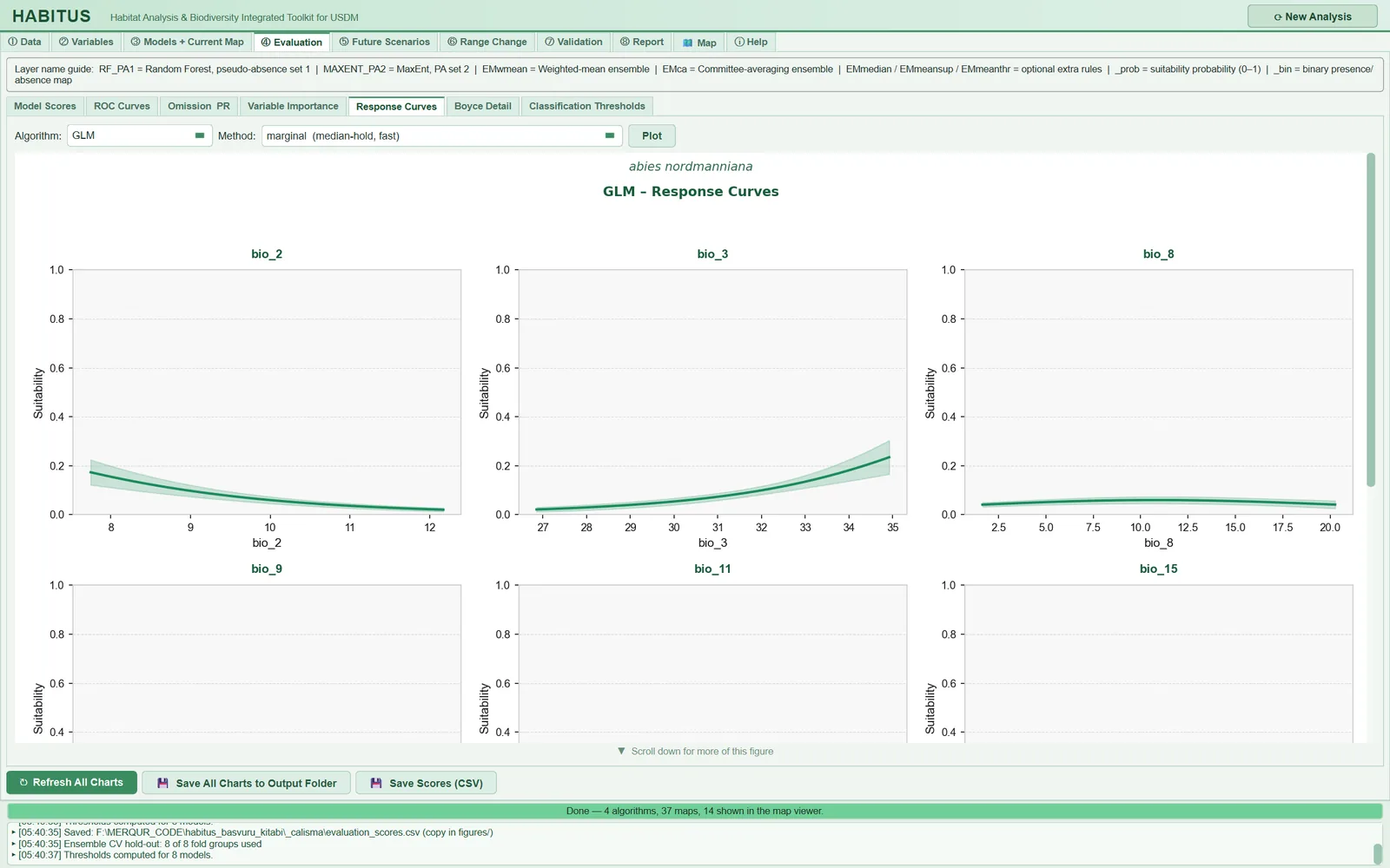
Figure 7.5. Response Curves sub-tab: Algorithm, Method and Plot controls; one panel per continuous predictor for the selected algorithm, the thick line is the mean response, the shading is the standard deviation across replicates; only the upper part of the second-row panels is visible, the curves lie in the region below 0.4 that becomes visible on scrolling.
| Name in the UI | What it does | Default | Options | Code |
|---|---|---|---|---|
Algorithm: |
Algorithm whose curves are drawn | first algorithm | algorithms in the run | tabs/tab_evaluation.py:654-655, 885-892 |
Method: |
Response curve method | marginal (median-hold, fast) |
marginal / partial / ice |
tabs/tab_evaluation.py:656-671 |
Plot |
Computes and draws the curves | — | — | tabs/tab_evaluation.py:672-673 |
7.7.1 Response curve method (Method)
What it does. Each continuous predictor is varied at 100 points between its 5th and 95th percentiles in the pooled data of all PA sets (presences and pseudo-absences) (compute_response_curves, sdm_core.py:8354-8510):
marginal: all other predictors are held at the median of the pooled data (the "median-hold" approach of biomod2).partial: partial dependence (PDP; Friedman 2001): in at most 500 seeded randomly selected real rows, the focal variable is set to each grid value and the predictions are averaged.ice: individual conditional expectation (ICE; Goldstein et al. 2015): a separate curve (thin lines) is drawn for each of 60 seeded randomly selected rows; the thick line is the mean of these curves, i.e. the PDP of those rows.
In every method, all fitted models of the algorithm (the CV runs of each PA set and the full-data model) are predicted separately; the thick line is their mean and the shading their standard deviation (sdm_core.py:8461-8506). For categorical predictors, one bar is drawn per class (other predictors at the median; variables with 2–60 classes) (sdm_core.py:8512-8553).
When and how to set it. marginal is fast and comparable with biomod2/maxnet outputs. If there are strong interactions or correlations between predictors, the median row may be an unrealistic combination of predictors; partial averages over the real data distribution. ice is used to see interactions: thin curves of differing shapes indicate that the effect of the focal variable depends on other variables.
Effect on results. Screen and evaluation_response_<ALGO>.png only. partial requires about 500 × 100 predictions, ice 60 × 100 predictions × the number of models; it is noticeably slow for MaxEnt and RF. The result is cached for the same run, method and algorithm; redrawing does not recompute (tabs/tab_evaluation.py:690-712).
Caution. The curves are computed without applying the Clamp predictors … setting of ③ Models (the prediction functions are called directly, sdm_core.py:8419-8437). The y axis is fixed to the range 0–1; with pseudo-absence data the probability scale is low, so the curves may look compressed (in the example run the GLM curves stay below 0.25). The shading of a curve shows the difference between CV and full-data models; it is not a confidence interval. The figure has 3 columns; with more than nine predictors, scroll the figure for the lower rows.
7.8 Boyce detail (Boyce Detail)
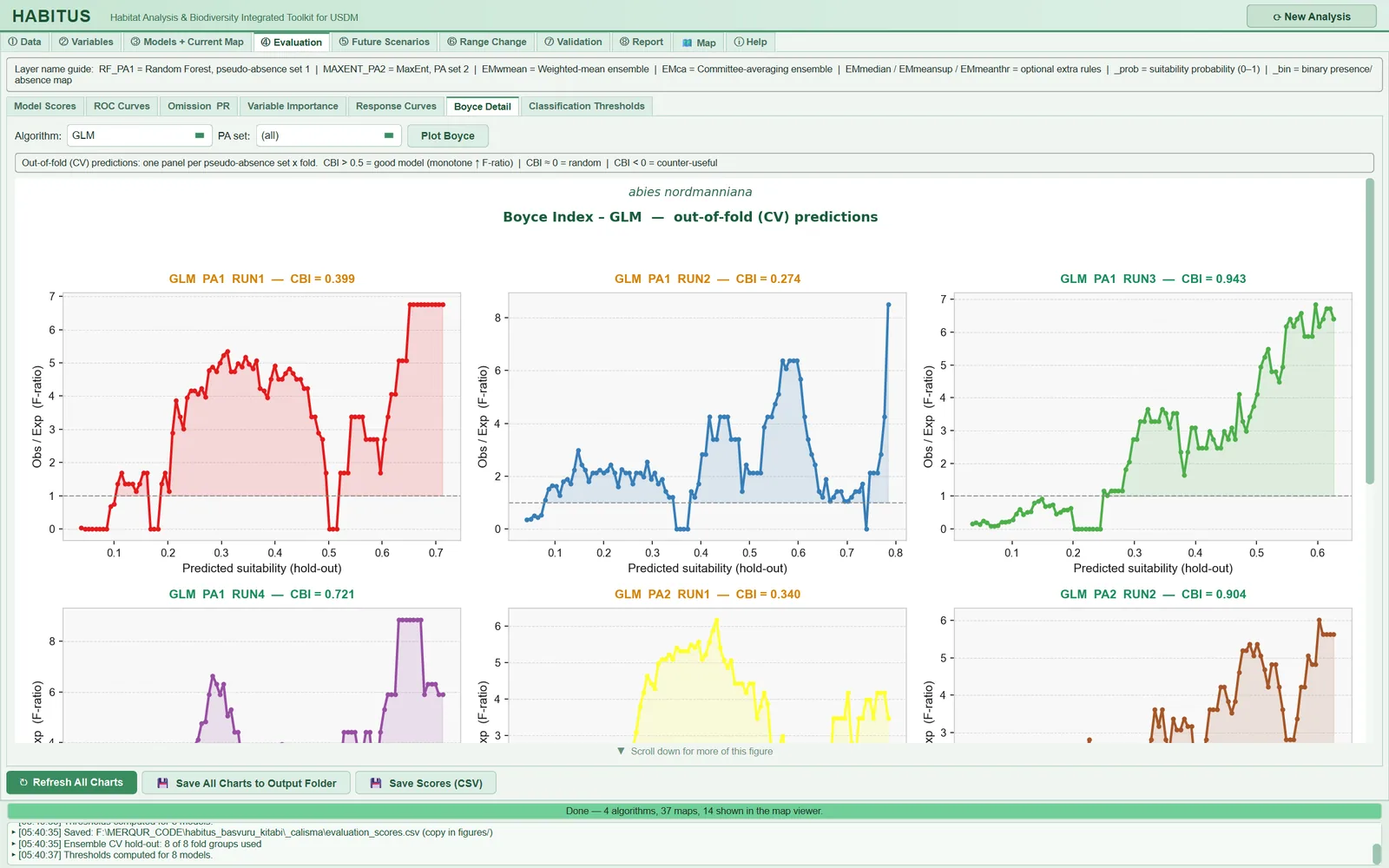
Figure 7.6. Boyce Detail sub-tab: one panel per PA set × fold group for the selected algorithm; P/E (F-ratio) curve, dashed line at level 1 and the CBI value of that fold in the title.
| Name in the UI | What it does | Default | Options | Code |
|---|---|---|---|---|
Algorithm: |
Algorithm | first algorithm | algorithms in the run | tabs/tab_evaluation.py:774 |
PA set: |
PA set to display | (all) |
(all), PA1, PA2, … |
tabs/tab_evaluation.py:775, 893-897 |
Plot Boyce |
Draws the panels | — | — | tabs/tab_evaluation.py:776-777 |
What it does. For each PA set × fold, a Boyce curve is drawn from the hold-out predictions: the x axis is the window midpoint, the y axis the ratio F=P_i/E_i; the region above 1 is shaded; the title colour is green for CBI ≥ 0.5, orange for 0–0.5 and red below 0 (cv_boyce_curves, sdm_core.py:6998-7015; tabs/tab_evaluation.py:791-847). The function called is the same call that produces the Boyce value in the score table; the CBI in the panel title matches the value in the table.
When and how to set it. In a good model, the P/E curve rises monotonically with suitability and lies below 1 at low suitability and above 1 at high suitability (Hirzel et al. 2006). A curve that falls after a peak indicates that the model assigns its highest values to too large an area; a flat curve indicates weak discrimination.
Effect on results. Screen and evaluation_boyce_<ALGO>.png. In the example run, the fold CBI values of GLM range from 0.274 (PA1 RUN2) to 0.943 (PA1 RUN3); in the RUN1 and RUN2 panels the P/E curve peaks at intermediate suitability and then falls.
Caution. The window width is one tenth of the prediction range (ecospat definition); in models with a very narrow prediction range (e.g. BIOCLIM) the windows fall very close to each other. If the number of presences per fold is small, the curve is stepped; read the CBI as the mean over folds, not from a single fold.
7.9 Classification thresholds (Classification Thresholds)
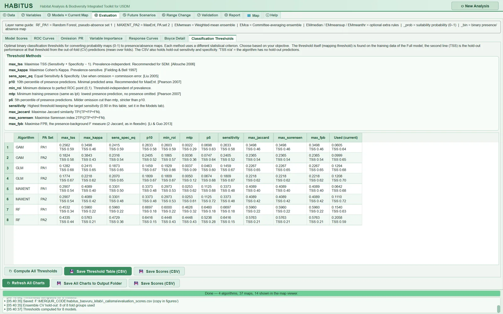
Figure 7.7. Classification Thresholds sub-tab: descriptions of the threshold rules and, for each full-data model, the threshold of each of the eleven rules (upper line) with the out-of-fold TSS at that threshold (lower line); the last column is the threshold used in the map.
| Name in the UI | What it does | Code |
|---|---|---|
Threshold Methods box |
Short definitions of the eleven rules | tabs/tab_evaluation.py:1132-1160 |
| Table | Rows: full-data model (algorithm × PA set); columns: 11 rules and Used (current) |
tabs/tab_evaluation.py:1162-1180 |
↻ Compute All Thresholds |
Recomputes the table | tabs/tab_evaluation.py:1183-1185 |
💾 Save Threshold Table (CSV) |
Writes figures/classification_thresholds.csv |
tabs/tab_evaluation.py:1316-1342 |
💾 Save Scores (CSV) |
Writes evaluation_scores.csv (§7.10) |
tabs/tab_evaluation.py:1188-1194 |
What it does. For each full-data model, a map threshold is found with each of the eleven rules (Chapter 6, §6.5.1), and two lines are written in the cell: the threshold and the mean over folds of the TSS this threshold gives on the out-of-fold predictions (tabs/tab_evaluation.py:1200-1314; sdm_core.py:7018-7037). The tooltip additionally shows the out-of-fold sensitivity and specificity at that threshold, the criterion value on the training data and the rule "pixel >= t -> Present (1)". The Used (current) column is the threshold actually used in the map. The CSV contains, for each rule, the threshold and the _holdout_Sens, _holdout_Spec, _holdout_TSS columns, the threshold used, the name of the rule and the number of folds.
When and how to set it. To support the choice of threshold rule: you see which rule gives a wider or narrower map while preserving out-of-fold TSS. The sensitivity column is always computed with a target of 0.90 (method description).
Effect on results. This table does not change the maps; the maps change when the rule is changed in ③ Models and the models are rerun.
Caution. The thresholds in this table and the threshold used in the map are found in different ways:
- The rule columns of the table are found from the full-data model's own (seen in training) predictions on the pooled data of all PA sets (
tabs/tab_evaluation.py:1217-1259). Used (current), in contrast, is the mean of the thresholds found in the CV folds in ③ Models with the selected threshold source (defaulttrain_cv) (sdm_core.py:5852-5853).
For this reason the max_tss column and Used (current) differ even for the same rule. In the example run, for GAM PA1 the max_tss column is 0.2562 (out-of-fold TSS 0.59) and the threshold used is 0.0605 (out-of-fold TSS 0.64). The difference grows for algorithms that memorise the training data: for RF PA1 the max_tss column is 0.4532 (out-of-fold TSS 0.34) and the threshold used is 0.1540 (out-of-fold TSS 0.63). To compare rules, look at the out-of-fold TSS in the lower line; do not read the threshold values as the map threshold.
7.10 Bottom buttons: refresh, save
| Name in the UI | What it does | Code |
|---|---|---|
↻ Refresh All Charts |
Updates the drop-down lists and recomputes all seven sub-tabs | tabs/tab_evaluation.py:851-872 |
💾 Save All Charts to Output Folder |
Writes all figures and the score table to the figures/ folder; can be cancelled |
tabs/tab_evaluation.py:939-1058 |
💾 Save Scores (CSV) |
Writes evaluation_scores.csv to the output root and a copy to figures/ |
tabs/tab_evaluation.py:1064-1108 |
What it does. Save All Charts … writes, in order, the score, ROC, omission/PR/calibration and importance figures; then, for each algorithm with CV models, the response curve figure (with the currently selected Method:) and the Boyce figure; and finally the score table (tabs/tab_evaluation.py:993-1030). Each figure is saved once as a 300 dpi PNG (tabs/tab_evaluation.py:923-937). When a figure is drawn on screen, it is also saved under the same name; therefore, before the button is pressed, the figures/ folder contains only the response and Boyce figures of the displayed algorithm (in the example run only evaluation_response_GLM.png and evaluation_boyce_GLM.png).
Caution. evaluation_scores.csv is written automatically when ③ Models finishes, when the tab is first opened and when the ensemble is rebuilt (tabs/tab_evaluation.py:1071-1081; tabs/tab_models.py:1840-1845); Save Scores (CSV) is only for repeating this manually. If there is no output folder, figures cannot be saved and "Output directory not set — cannot save figure." is written to the log. The information window after saving mentions a figures/response_curves/ subfolder; no such folder is created, and a single combined figure is written per algorithm.
7.11 Outputs and what passes to the next step
In the <output>/figures/ folder:
evaluation_model_scores.png,evaluation_roc_curves.png,evaluation_omission_pr_calibration.png,evaluation_variable_importance.pngevaluation_response_<ALGO>.png,evaluation_boyce_<ALGO>.pngevaluation_omission_pr_calibration.csv,classification_thresholds.csv,evaluation_scores.csv(copy)
evaluation_scores.csv in the output root. This tab does not change models, thresholds or maps; ⑧ Report uses the same score table and figures (Chapter 11).
7.12 Expert questions
Q1. Are the ROC, omission and Boyce curves on this tab based on independent data? Is the model tested on its training data?
Answer: The curves are drawn only from the CV hold-out predictions saved in ③ Models (modeler.cv_holdout; sdm_core.py:5547-5556); no new split is made and no predictions are made on training rows (sdm_core.py:6926-6932). The degree of independence depends on the CV design in ③ Models: with spatial blocks, the tests are geographically separate from training; with the random design they are not. The exceptions are the response curves and the threshold columns of the Classification Thresholds table.
Q2. Is the AUC reported for the ensemble (EMwmean) computed from the ensemble map?
Answer: No. The ensemble rows and ROC panels are produced by combining, in each fold, the CV models that have not seen that fold with the ensemble rule and scoring them only on that fold; member selection and weights come from the scores of the other folds (sdm_core.py:6516-6696). The note on the scores sub-tab states this explicitly: "… they are NOT computed from the ensemble map." (tabs/tab_evaluation.py:269-274).
Q3. At how many thresholds and on which data is TSS computed; is it comparable with ecospat or biomod2?
Answer: TSS is computed on the test fold, at the threshold that the selected rule (default max_tss) finds on the inner out-of-fold predictions of the training rows (sdm_core.py:1193-1217). biomod2 and ecospat.max.tss usually optimise the threshold on the evaluation data itself; this "oracle" threshold raises TSS. If Test-fold threshold: = test is selected in ③ Models, HABITUS follows the same path and the numbers become comparable; however, this choice is optimistic (Chapter 6, §6.5.2).
Q4. Is the Boyce index exactly the same as in ecospat?
Answer: The default ecospat formula is a line-by-line port of the ecospat.boyce function (ecospat 4.1.4): window width 1/10 of the prediction range, 101 positions, closed windows, removal of consecutive repeated P/E values, and Spearman correlation (sdm_core.py:475-543). The difference lies in the choice of the fit set: HABITUS uses all rows of the evaluation fold (test presences and test pseudo-absences) (sdm_core.py:605-610); in ecospat, fit is in most applications the raster predictions of the whole study area. The values therefore match exactly for the same predictions, and approximately for the full map.
Q5. How is the calibration slope computed, and what does it mean with pseudo-absence data?
Answer: It is the slope of the logistic regression (practically unpenalised, C = 1e12) of the observation on the logit of the prediction; predictions are clipped to the range [10^{-6}, 1-10^{-6}], and at least 10 rows and two classes are required (sdm_core.py:989-1013; Pearce and Ferrier 2000). With pseudo-absence data, the scale of the probability depends on the PA:presence ratio; the slope is an indicator not of the true probability of presence but of the model's over- or underconfidence on out-of-fold data. A slope much smaller than 1 (overfitting) is meaningful in comparisons between algorithms.
Q6. Why does OR_10p sometimes come out as 0, and is this a good result?
Answer: Not always. If the omission threshold is equal to or below the lowest prediction of the evaluation set, no presence can fall below the threshold; omission is 0 by construction. This case is flagged with OR_10p_degenerate = 1; if it occurs in at least half of the folds, a warning is written for the algorithm (sdm_core.py:1100-1114, 5787-5816). It is usually seen with BIOCLIM, shallow CART and strongly regularised GLMNET; the omission of these algorithms should not be compared with that of the others.
Q7. Which method is used to compute variable importance; is it like MaxEnt's percent contribution?
Answer: No, it is permutation importance: a predictor is shuffled on the test fold and the drop in AUC is measured (sdm_core.py:5564-5636). MaxEnt's "percent contribution" and "permutation importance" outputs are normalised to percentages and computed on the training data; HABITUS does not normalise and computes on the test fold. For scikit-learn models, because of the fixed seed, the Variable importance reps: repetitions give the same result; the effective repetition is n_repeats = 3.
Q8. From which models and which data are the response curves produced?
Answer: From all fitted models of the algorithm (the CV runs of each PA set and the full-data model); the thick line is their mean, the shading their standard deviation (sdm_core.py:8461-8506). The range of the variable and the median row are taken from the pooled presence and pseudo-absence rows of all PA sets; the range is the 5th–95th percentile, and there is no extrapolation at the ends (sdm_core.py:8405-8457). The default approach in biomod2's bm_PlotResponseCurves function is also to hold the other variables at a fixed value (the median); because the variable range and summarising details are not the same in the two programs, the curves may be similar in shape but not numerically identical.
Q9. When do marginal, PDP and ICE give different results?
Answer: When there are interactions or strong correlations between predictors. Marginal shows only the neighbourhood of the median row; PDP averages over real data rows (Friedman 2001); ICE shows the curve of each row separately and reveals the heterogeneity that PDP hides by averaging (Goldstein et al. 2015). In a linear additive model (e.g. a GLM without interactions) all three give the same shape, though their levels may differ; they diverge in tree models and in GLMs with interactions terms.
Q10. Why is max_tss in the Classification Thresholds table not the same as the threshold in the map?
Answer: The table finds the threshold from the full-data model's predictions (seen in training) on the pooled data of all PA sets (tabs/tab_evaluation.py:1217-1259); the threshold in the map, in contrast, is the mean of the thresholds found in the CV folds according to the threshold source (sdm_core.py:5852-5853). In the example run, for RF PA1 the table gives 0.4532 and the map 0.1540; because RF's training predictions are close to 1 at presences, the table threshold comes out high and out-of-fold TSS drops to 0.34, whereas the map's threshold gives 0.63. The reliable part of the table is the out-of-fold TSS in the lower line.
Q11. Is the difference between algorithms significant? Is a test provided?
Answer: No, there is no statistical comparison test. The program gives the mean, SD and range over folds and PA sets (sdm_core.py:5883-5919), and the charts show the distribution. Because the folds derive from the same data, they are not independent; a simple t test would not be valid either. In the example run, the difference between folds of the same algorithm (GLM PA1 ROC 0.790–0.941) is larger than the difference between algorithms; in this situation it is more defensible to include several algorithms in the ensemble than to rank them.
Q12. How does an algorithm run without ESM or CV appear on this tab?
Answer: Algorithms without out-of-fold predictions are listed with a "Not shown" note in the ROC, omission and Boyce figures (sdm_core.py:6872-6876, 6974-6977); the Classification Thresholds cells show TSS n/a. ESM's hold-out predictions are saved and appear normally; only because it does not produce inner out-of-fold training predictions may its threshold source be labelled differently (Chapter 6, §6.5.2).
7.13 Common mistakes and pitfalls
- Taking the distribution in the
Model Scoreschart for the spread between folds: the chart also includesFull(CV mean) and ensemble rows. - Not being able to see a model with TSS below 0.3 in the chart: the axis starts at 0.3; read the value in the table or CSV.
- Taking the threshold values in the
Classification Thresholdstable for the map threshold; the map threshold is theUsed (current)column. - Interpreting calibration and precision values as true probabilities of presence; the scale depends on the PA:presence ratio.
- Reporting the shading of a response curve as a confidence interval; it is the SD across replicates.
- Expecting response and Boyce figures for every algorithm in the
figures/folder without usingSave All Charts …. - Running with
Variable importance reps:= 0 and searching for why the importance chart is empty. - Assuming that clamping (
Clamp) is applied to the response curves.
7.14 References
Allouche, O., Tsoar, A., Kadmon, R., 2006. Assessing the accuracy of species distribution models: prevalence, kappa and the true skill statistic (TSS). Journal of Applied Ecology 43, 1223–1232. https://doi.org/10.1111/j.1365-2664.2006.01214.x
Fielding, A.H., Bell, J.F., 1997. A review of methods for the assessment of prediction errors in conservation presence/absence models. Environmental Conservation 24, 38–49. https://doi.org/10.1017/S0376892997000088
Friedman, J.H., 2001. Greedy function approximation: A gradient boosting machine. The Annals of Statistics 29, 1189–1232. https://doi.org/10.1214/aos/1013203451
Goldstein, A., Kapelner, A., Bleich, J., Pitkin, E., 2015. Peeking inside the black box: Visualizing statistical learning with plots of individual conditional expectation. Journal of Computational and Graphical Statistics 24, 44–65. https://doi.org/10.1080/10618600.2014.907095
Hirzel, A.H., Le Lay, G., Helfer, V., Randin, C., Guisan, A., 2006. Evaluating the ability of habitat suitability models to predict species presences. Ecological Modelling 199, 142–152. https://doi.org/10.1016/j.ecolmodel.2006.05.017
Li, W., Guo, Q., 2013. How to assess the prediction accuracy of species presence–absence models without absence data? Ecography 36, 788–799. https://doi.org/10.1111/j.1600-0587.2013.07585.x
Pearce, J., Ferrier, S., 2000. Evaluating the predictive performance of habitat models developed using logistic regression. Ecological Modelling 133, 225–245. https://doi.org/10.1016/S0304-3800(00)00322-7