1. Introduction and workflow
Scope: main window · Code: main.py (start-up), main_dialog.py (main window, tab locks, log), threads.py (background jobs), run_config.py (seed and run record), tabs/tab_data.py (seed and output folder fields)
1.1 What HABITUS is
HABITUS is a desktop program for species distribution modelling (SDM) that requires no coding. It takes the coordinates of the locations where a species occurs (presence records, CSV) and environmental raster layers on the same grid; from these it builds a habitat suitability model, evaluates the model by cross-validation, produces maps for current and future climate, computes the change in area between two maps and gathers all steps into an HTML report (Elith and Leathwick, 2009).
Computations are done in Python: with the scikit-learn, xgboost, lightgbm, catboost, pygam and elapid libraries and NumPy. No R installation is needed and no R packages are called. In this book, R packages (biomod2, dismo, ENMeval, blockCV, maxnet, ecospat) are mentioned only for comparison.
Two tasks remain outside the program. The first is the collection and cleaning of the presence records. The second, when no study boundary is given, is bringing the rasters onto a common grid: all continuous and categorical rasters must have the same dimensions, cell size, origin and coordinate reference system (CRS). HABITUS checks this on loading and names the file that differs, but does not resample it (Chapter 2).
Note: The UI is in English. In this book, button, box and tab names are given in
codeformat exactly as they appear in the UI.
1.2 How to use this book
The book follows the program's tabs from left to right. Every chapter has the same layout: the tab's place in the workflow, the screen layout, field groups and parameter tables, a four-part explanation for every parameter that affects the result (What it does, When and how to set it, Effect on results, Caution), outputs, expert questions, common mistakes and references.
- The default values and ranges in the parameter tables were read from the source code; the
Codecolumn gives the location in the formfile.py:line. - The screenshots and the numbers given in the text come from an example run: Abies nordmanniana (626 records), WorldClim 2.1 bioclimatic variables (2.5 minutes), future scenario MPI-ESM1-2-HR SSP5-8.5 2081-2100, algorithms GLM, GAM, RF and MAXENT. These numbers are there to illustrate the UI; they are not a conclusion about the ecology of the species.
- A first-time reader should read this chapter and then Chapters 2-6 in order. A reader looking for the meaning of a setting can go directly to the parameter table of the relevant chapter. The full list of output files, the run record and troubleshooting are in Chapter 12.
Distribution of chapters over the tabs:
| Chapter | Tab | Topic |
|---|---|---|
| 2-3 | ① Data |
Records, rasters, study boundary, pseudo-absence and background |
| 4 | ② Variables |
VIF, correlation, advanced multicollinearity analysis, variable selection |
| 5-6 | ③ Models + Current Map |
Algorithms, cross-validation, threshold, ensemble, Tuning, current map |
| 7 | ④ Evaluation |
Scores, ROC, omission, variable importance, response curves, Boyce, thresholds |
| 8 | ⑤ Future Scenarios |
Projection to future climate, extrapolation diagnostics |
| 9 | ⑥ Range Change |
Loss, gain and stable area |
| 10 | ⑦ Validation |
Accuracy against independent maps or points |
| 11 | ⑧ Report |
HTML report, ODMAP, batch run on a multi-species file |
| 12 | 🗺 Map, ⓘ Help |
Record map, help, output files, run record, troubleshooting |
1.3 Installation and platforms
HABITUS runs on three desktop platforms. The packaged release carries its own Python interpreter and all libraries; no separate Python installation is needed.
| Platform | Package | Installation |
|---|---|---|
| Windows | Installer (HABITUS_Setup_v*.exe) or portable ZIP |
Run the installer; the program opens from the Start menu and the desktop shortcut. At the SmartScreen warning, choose More info and Run anyway |
| macOS | .dmg disk image (Apple Silicon and Intel) |
Drag HABITUS.app into the Applications folder; on first launch, right-click and Open |
| Linux | AppImage or tar.gz |
Give the AppImage file execute permission and run it; in the tar.gz archive the program is started with run_habitus.sh |
| From source | main.py |
python main.py in a Python environment where the dependencies are installed |
The minimum Python version required to run from source is 3.10 (pyproject.toml:11). If the optional algorithm libraries (xgboost, lightgbm, catboost, pygam, elapid) are not installed, the program still opens; the corresponding algorithms are marked as unavailable in the ③ Models tab (main.py:365-367). Detailed system requirements are in Chapter 12.
Self-test. If the packaged program is given the --selftest argument (HABITUS.exe --selftest, from source python main.py --selftest), no window opens; the program tests the coordinate database, a coordinate transformation, vector reading, writing and reading a GeoTIFF, which algorithms can be run, and Qt, and prints a report (main.py:195-197, selftest.py). If --require-algorithms GLM,MAXENT is added, the test is counted as failed when any of the named algorithms is missing (selftest.py:368-376). This is the quickest way to make sure an installation works.
1.4 Start-up
When the program starts, a splash screen appears first. Meanwhile the scientific libraries are loaded one by one and the splash screen shows the name of the library being loaded: plotting (matplotlib), tables (pandas), SciPy, raster reading (rasterio), vector layers, machine learning, XGBoost, LightGBM, CatBoost, MaxEnt (elapid) and GAM (main.py:223-235). On a cold start this may take a few seconds; loading is deliberately done before the window so that the screen does not stay blank.
At start-up the program also does the following:
- It checks the coordinate transformation database (
proj.db). If an old database left over from another installation (e.g. PostGIS) is defined in the environment, it selects the program's own copy (main.py:88-163). - On Linux and macOS it resets the character and numeric locale to the neutral C locale, so that under a Turkish locale the raster library does not go wrong in upper/lower case comparisons. The UI is not affected; this step is not applied on Windows (
main.py:293-315). - It opens the crash log (Chapter 12).
- It starts a check for a new release in the background; the result appears on the
ⓘ Help>Aboutpage (main_dialog.py:130-148).
The initial size of the main window is 95% of the screen width and 92% of its height, at most 1600 x 1000 logical pixels (main_dialog.py:113-121). The window can be resized; every tab is inside a scroll area, and on a narrow screen the content scrolls (main_dialog.py:183-193).
1.5 Layout of the main window
The main window consists of four regions (main_dialog.py:150-217):
- Title bar. On the left the program name and subtitle, on the right the
⟳ New Analysisbutton (§1.5.1). - Tab bar. Eight numbered workflow tabs plus
🗺 Mapandⓘ Help(§1.6). - Tab content. The screen of the selected tab; described in Chapters 2-12.
- Bottom status bar. Progress bar and log panel (§1.7).
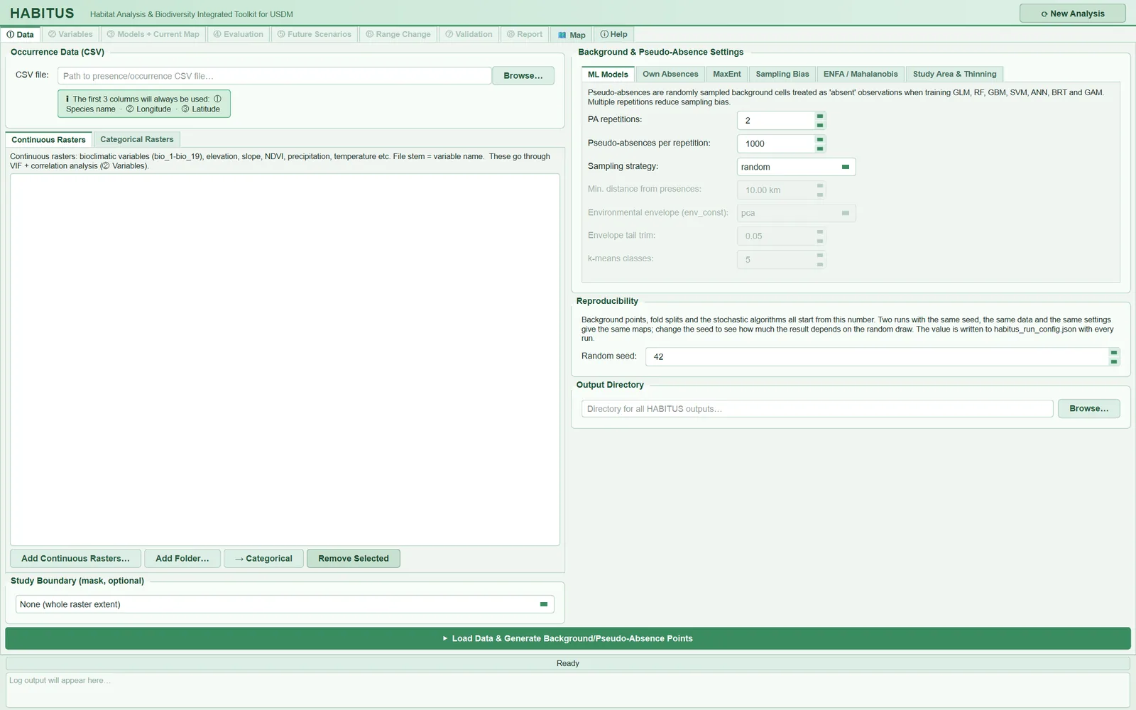
| Name in the UI | What it does | Default | Range / options | Code |
|---|---|---|---|---|
⟳ New Analysis |
Asks for confirmation; deletes all data, models and results from memory, locks the tabs, returns to ① Data |
— | button; Yes / No in the confirmation dialog (default No) |
main_dialog.py:159-163, 241-249, 303-419 |
| Tab bar | Workflow steps; tabs after an unfinished step are greyed out and cannot be clicked | ① Data, 🗺 Map, ⓘ Help open |
ten tabs | main_dialog.py:186-199 |
| Progress bar | Shows the step and percentage of the running job; green when the job finishes, red on error | Ready, 0% |
0-100% | main_dialog.py:205-208, 659-703 |
| Log panel | Writes every message with its time; the same lines also go to the session log file | empty (Log output will appear here…) |
read-only | main_dialog.py:209-216, 790-801 |
Random seed (① Data > Reproducibility) |
Starting number of all random operations | 42 | 0-2147483647 | tabs/tab_data.py:242-249 |
Output Directory (① Data) |
Folder to which all outputs are written | empty; filled automatically when a CSV is selected | any folder | tabs/tab_data.py:253-259, 1125-1162 |
Output Directory (for saving map files) (③ Models) |
Folder to which models and maps are written; if empty, uses the folder in ① Data | automatic from ① Data | any folder | tabs/tab_models.py:679-686, 1338-1348, 1470-1477 |
1.5.1 ⟳ New Analysis
- What it does. If
Yesis answered to the question "This will clear all loaded data, models, and results. Proceed?", the program stops running background jobs (waiting at most 1.5 seconds), resets the shared state, clears the three map viewers, locks all tabs from② Variablesto⑧ Reportand returns to① Data. In① Datathe presence CSV path, the raster lists and theOutput Directoryfield are emptied; the session log is closed (main_dialog.py:303-419). - When and how to set it. Used when switching to another species or to an entirely different data set. It is not needed to change just one setting for the same species and run again; re-running the relevant step is enough (§1.6.2).
- Effect on results. Everything in memory is deleted. The settings in the tabs (seed, number of pseudo-absences, algorithm choices, etc.), however, are not deleted; the new analysis starts with the previous settings. Because
Output Directoryis emptied, a new analysis folder is created when a new CSV is selected (§1.9). - Caution. Files on disk are not deleted. The folder of the previous analysis remains as it is.
1.6 Tab bar and lock scheme
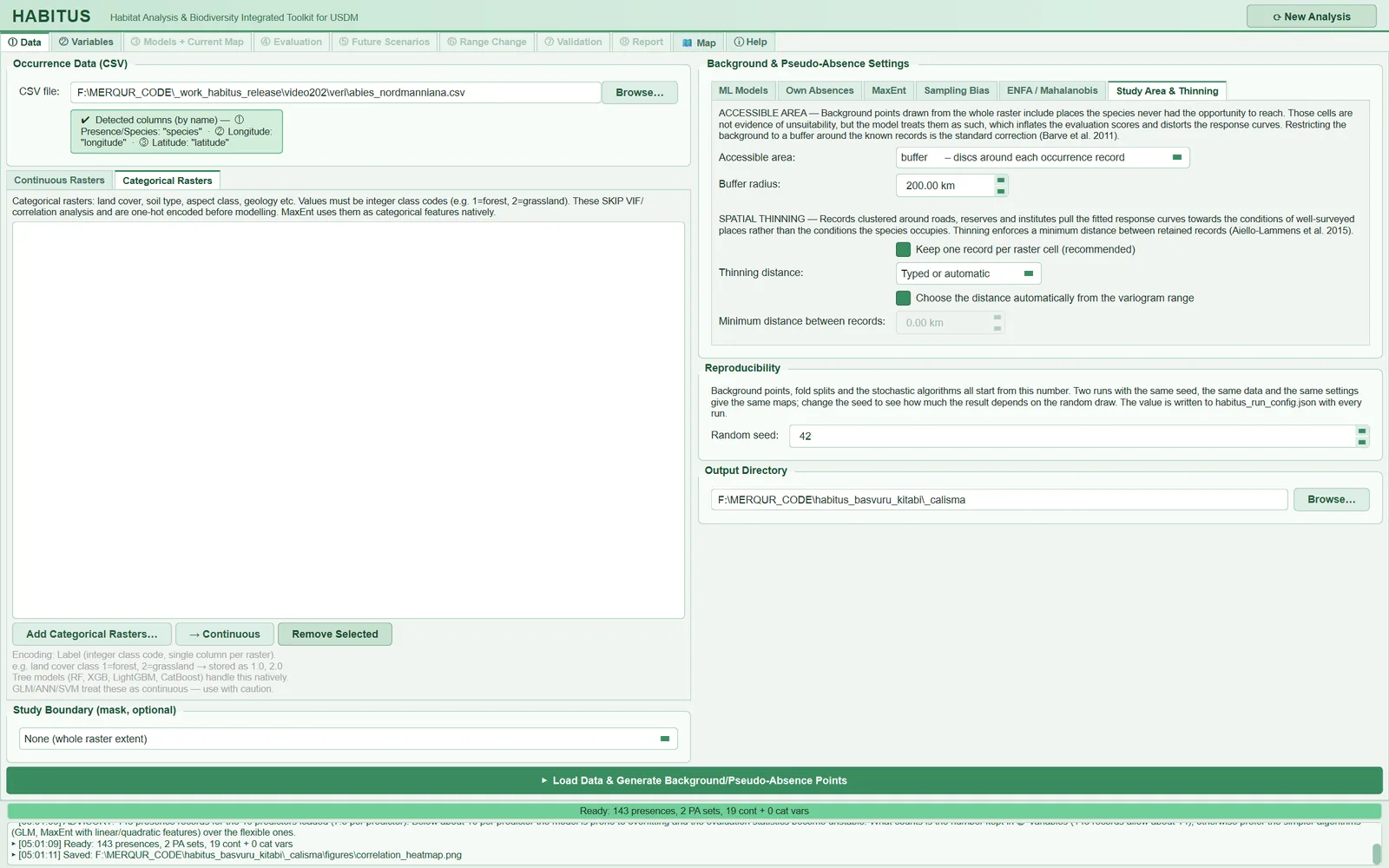
The tabs follow the order of the workflow. When the program opens, only ① Data, 🗺 Map and ⓘ Help are enabled; the seven tabs from ② Variables to ⑧ Report are locked (main_dialog.py:198-199). When a step finishes successfully, the next tab is unlocked and in most cases the program switches to that tab.
| Completed step | Tabs unlocked | Where the program switches | Code |
|---|---|---|---|
① Data: Load Data & Generate Background/Pseudo-Absence Points |
② Variables |
② Variables |
tabs/tab_data.py:1759-1760 |
② Variables: confirming the variable selection |
③ Models + Current Map |
③ Models, Algorithm Settings sub-tab |
tabs/tab_vif.py:1206-1208 |
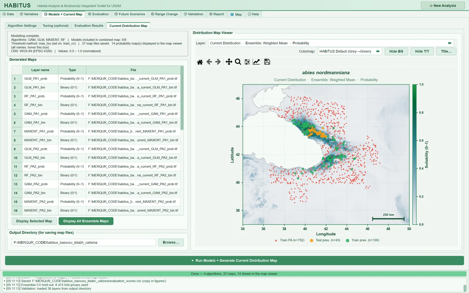
③ Models: Run Models + Generate Current Distribution Map |
④ Evaluation, ⑤ Future Scenarios, ⑥ Range Change, ⑦ Validation, ⑧ Report (together) |
Current Distribution Map sub-tab within ③ Models |
tabs/tab_models.py:1848-1852 |
⑤ Future Scenarios: projection |
(already open) ⑥ Range Change, ④ Evaluation |
tab does not change | tabs/tab_projection.py:672-673 |
After ③ Models has finished, the order ④-⑧ is not mandatory: for example, ⑦ Validation or ⑧ Report can be used without running ⑤ Future Scenarios. ⑥ Range Change needs two binary maps; if there is no future map, only a comparison between current maps is possible (Chapter 9). When the other species of a multi-species file are processed with the batch run in ⑧ Report, all tabs are unlocked (batch_species.py:215-217).
1.6.1 Tab bar summary
The whole workflow is in the following table. The "Main output" column gives the principal files written to the output folder; the full catalogue is in Chapter 12.
| Tab | What it does | Main output | Chapter |
|---|---|---|---|
① Data |
Reads and filters the records (one record per cell, thinning), loads the rasters and checks the grid, defines the accessible area, generates pseudo-absence and MaxEnt background points | accessible_area.tif, optional background_maxent.csv; training tables in memory |
2-3 |
② Variables |
Ranks variables by VIF and correlation; the user selects and confirms continuous and categorical variables; optional condition number, PCA, LASSO, Ridge | correlation heat maps, VIF plot, high_correlation_pairs.csv, variable_priority_ranking.csv in figures/ |
4 |
③ Models + Current Map |
Trains the selected algorithms with cross-validation, sets the threshold and builds the ensemble, writes the current-climate map; optional Tuning | probability, binary and uncertainty rasters in the current/ folder; evaluation_scores.csv; occurrence_train.csv, occurrence_test.csv; habitus_run_config.json |
5-6 |
④ Evaluation |
Scores, ROC, omission and calibration, variable importance, response curves, Boyce, threshold tables | figures/evaluation_*.png, figures/classification_thresholds.csv |
7 |
⑤ Future Scenarios |
Applies the models to future climate rasters; extrapolation maps (ExDet, optional MESS) | probability, binary, NT1, NT2, MIC rasters in the <scenario>/ folder; projection_options.json |
8 |
⑥ Range Change |
Compares two binary maps: loss, gain, stable | <species>_<analysis name>_SRC.tif and area table |
9 |
⑦ Validation |
Compares the model with an independent reference map or points | reclassified rasters in the validation/ folder; optional report and point file |
10 |
⑧ Report |
Gathers all steps into a scientific HTML report; exports the ODMAP protocol; runs the other species of a multi-species file | <species>_HABITUS_report_<time>.html, odmap_protocol.md/.csv, batch_summary.csv |
11 |
🗺 Map |
Shows the inputs (records, excluded records, own absences, boundary) on an online basemap; study area figure for publication | <species>_study_area.png (optional) |
12 |
ⓘ Help |
English user guide and update check | — | 12 |
1.6.2 Re-running a step deletes the later results
HABITUS does not keep the results that follow a step with the old input when the input of that step changes. There are two deletion paths:
- If
① Datais re-run (when data have been loaded before), the program, without asking for confirmation, stops running model, projection and change jobs, deletes the variable selection, models, ensemble, projections, change results, Tuning results, evaluation plots and validation results held in memory, and locks all tabs from② Variablesto⑧ Report. "Data inputs changed — all previous results cleared. Re-running data formatting…" is written to the log (tabs/tab_data.py:1396-1397,main_dialog.py:421-526). - If the selection in
② Variablesis re-confirmed and the models have already been run, the "Re-confirm Variable Selection" dialog asks: "Confirming now will discard all existing models, maps, projections, and evaluation results so everything is recomputed from scratch." IfYesis answered, the models and all later results are deleted;① Data,② Variablesand③ Modelsstay open,④-⑧are locked. "Variable selection changed — downstream results cleared. Re-run Models to continue." is written to the log (tabs/tab_vif.py:1170-1185,main_dialog.py:528-594).
When ③ Models is re-run, the tabs are not locked; the new results replace the old ones.
Caution: Deletion applies only to the program's memory. Files in the output folder are not deleted; a new run overwrites files with the same name. Rasters left from the first run by an algorithm not selected in the second run, and old PNGs in
figures/, remain in the folder. Because⑧ Reportreads all PNGs infigures/and⑦ Validationreads the layers in the output folder (tabs/tab_report.py:578-587), using a new output folder for every run with changed settings is the safest course.
1.7 Bottom status bar: progress bar and log
Progress bar
While a long job is running, the bar shows the current step and the percentage (e.g. "Reading raster 3 of 19: bio_11.tif 12%"). The bar only moves forward during the job; it reaches 100% only when the job has really finished. On completion the bar turns green and summarises the result (e.g. "Done — 4 algorithms, 37 maps, 14 shown in the map viewer"); on error it turns red and reads "Failed — see the message" (main_dialog.py:659-703, 755-788).
While a job is running, the button that started it is disabled and its text changes; a second click does not start a second job. The button is re-enabled when the job ends successfully, with an error or by cancellation (main_dialog.py:707-788). The ⑦ Validation and ⑧ Report jobs run in the UI thread; during this time a small "HABITUS" window shows the current step and the cursor changes to the wait cursor (main_dialog.py:712-753).
Log panel
Every message of the program appears in the log panel in the form ▸ [HH:MM:ss] message and the panel automatically scrolls to the last line (main_dialog.py:790-793). The log contains: the progress messages of every step, warnings (⚠, WARNING:), informational notes that affect interpretation (ADVISORY:), the path of every saved file (Saved: …) and the last line of errors (ERROR: …).
From the moment the output folder is known, the same lines are also written to the session log file (main_dialog.py:612-645, 794-801):
- The file name is
<species>_<YYYYMMDD_HHMMSS>.log. If the species name is not known at that moment (e.g. if the output folder was selected manually), the name becomeshabitus_<YYYYMMDD_HHMMSS>.log. The log file of the example run is namedhabitus_20261121_050108.log. - The file begins with "HABITUS Analysis Log", the species name and the start time;
New Analysisor closing the window closes the file with a "Closed" line. - If the output folder changes (e.g. the next species in a multi-species file), the old log is closed and a new one is opened in that folder.
- When an error occurs, the full error message is appended to the log under a
--- ERROR ---header; the error dialog also shows the path of the log file (main_dialog.py:806-827).
The error dialog ("HABITUS Error") shows the last line of the error as its title and, for recognised errors, a plain suggestion. Show details opens the full text, Copy full message copies all of it to the clipboard (error_dialog.py:30-56, 80-182). When reporting a problem, this text and the session log should be sent together.
1.8 Progress, cancellation and closing the window
Data preparation, modelling, projection, range change, Tuning, raster folder scanning and the update check run in a background thread; the window does not freeze meanwhile and other tabs can be browsed (threads.py:1-23).
Cancellation is cooperative: when a stop is requested, a flag of the job is set and the job stops at its next progress report; a cancelled job reports neither a result nor an error (main_dialog.py:37-74, threads.py:34-63). There is no separate "stop" button for the ③ Models, ① Data and ⑤ Future Scenarios jobs; a running job is stopped in these ways:
⟳ New Analysis(waits at most 1.5 seconds),- re-running
① Dataor re-confirming the variable selection (stops the downstream jobs), - closing the window.
The Tuning (optional) sub-tab has its own Cancel button (Chapter 6); the batch figure saving in ④ Evaluation can also be cancelled from the progress dialog (Chapter 7).
If the window is to be closed while a job is running, the program asks: "Data formatting, Models still running — close anyway? The unfinished work is discarded." (with the names of the running jobs; default No). If Yes is answered, the jobs are cancelled and the program waits at most a few seconds (main_dialog.py:284-301, 596-608).
Note: Cancellation takes effect at a progress report. A single long computation (e.g. training a single model on a large data set) continues in the background until it finishes; its result does not reach the window, but it uses the processor for that time (
main_dialog.py:266-282).
1.9 Output folder and automatic analysis folder
All outputs are written to a single folder: ① Data > Output Directory.
- Automatic folder. If a presence CSV is selected while
Output Directoryis empty, the program creates a folder namedDocuments/HABITUS/<species>_<YYYYMMDD_HHMMSS>in the user's documents folder and writes it into the field; "Analysis folder auto-created: <path>" appears in the log. The species name is the most frequent value in the species column of the CSV (in a GBIF file thespeciescolumn is recognised by its name); for a multi-species file the folder takes the name of the CSV file. If there is no documents folder, the home folder is used; characters other than letters, digits, dots and hyphens in the name are converted to underscores (tabs/tab_data.py:1125-1162,main_dialog.py:831-853). - Manually selected folder. A folder selected with
Browse…or typed in manually is used as it is; no automatic folder is created. - Multi-species file. Each species is written to its own subfolder under the output folder (
tabs/tab_data.py:1115-1123; Chapter 2). ③ Modelsfolder. TheOutput Directory (for saving map files)field in③ Modelsis filled automatically with the folder from ① Data. If the user enters another folder here, the modelling outputs and all subsequent steps (and the session log) move to that folder (tabs/tab_models.py:1338-1348,1470-1477).
1.9.1 Output Directory
- What it does. Sets where raster maps, tables, figures, the run record, the session log and the report are written. If it is empty,
Load Data & Generate Background/Pseudo-Absence Pointsdoes not run and shows the message "Please specify an output directory." (tabs/tab_data.py:1370-1371). - When and how to set it. A separate folder is recommended for each analysis; the automatic folder provides this by itself with a time stamp. If comparative runs with different settings are to be made for the same species, each run should be given a new folder.
- Effect on results. It does not change the computed numbers. But writing to the same folder a second time overwrites
habitus_run_config.json,evaluation_scores.csvand the rasters, and files left over from the previous run may appear in the report (§1.6.2). - Caution. If
evaluation_scores.csvhas been edited manually, it is backed up asevaluation_scores.<time>.bak.csvbefore being overwritten (sdm_core.py:6764-6776); other files are not backed up. If a file in the output folder is open in another program (e.g. a GIS program or a spreadsheet), writing may fail with "Permission denied".
1.10 Random seed and reproducibility
The Random seed in the ① Data > Reproducibility group is the single starting number of the whole analysis. The description in the UI: "Background points, fold splits and the stochastic algorithms all start from this number. Two runs with the same seed, the same data and the same settings give the same maps; change the seed to see how much the result depends on the random draw." (tabs/tab_data.py:234-249).
1.10.1 Random seed
- What it does. When
① Datais run, the seed is applied before anything random is done (tabs/tab_data.py:1505-1510,sdm_core.py:115-119). NumPy's global random number generator and Python'srandommodule are initialised with this number; if thePYTHONHASHSEEDenvironment variable is not defined, it is set to this number (run_config.py:31-50). Background and pseudo-absence sampling, the assignment of cross-validation folds and all stochastic algorithms (RF, GBM, BRT, MaxEnt, etc.) are derived from the same value. When modelling has finished, the seed is written to therandom_seedfield of thehabitus_run_config.jsonfile (tabs/tab_models.py:2071,run_config.py:141). - When and how to set it. For publication, the default 42 or any fixed value is sufficient; what matters is that the value is reported. To see how much the result depends on the random draw, the same analysis can be repeated with several different seeds (e.g. 1, 2, 3) and the scores and maps compared.
- Effect on results. Two runs with the same data, the same settings and the same seed give the same pseudo-absence points, the same folds and the same maps. If the seed changes, the points and folds change; the scores and maps vary by the amount of this variability. In species with few records this variation can be marked.
- Caution. The seed is read when
① Datais run. After changing the seed, re-running only③ Modelsdoes not apply the new seed:① Datamust be re-run (which also deletes the later results, §1.6.2). Equality at bit level is not guaranteed; in multi-threaded computations (e.g. RF) the order of summation can produce small differences in the last digit.
1.11 Example data
A ready-made example data package (habitus_sample.zip) for trying out the program can be downloaded from the program's release page. The package contains the presence records of one species, the 19 bioclimatic variables, additional layers such as elevation and NDVI, categorical layers (aspect, slope), several climate scenarios and periods, and a reference distribution map for validation (README.md, "Sample Data"). The ornek_veri folder in the source tree additionally contains Pinus brutia records together with two synthetic absence files generated by rules for trying out the Own Absences sub-tab, and a calibration area polygon; the synthetic files are not field data and must not be used in an analysis intended for publication (ornek_veri/OKUBENI.md).
The screenshots in this book, however, were taken with the Abies nordmanniana data (§1.2).
Shortest path for a first try. (1) In ① Data, select the CSV with Browse…; the output folder is created automatically. (2) Add the bioclimatic folder with Add Folder…. (3) Leave the other settings at their defaults and press Load Data & Generate Background/Pseudo-Absence Points. (4) In ② Variables, confirm the suggested variables. (5) In ③ Models, select a few algorithms and press Run Models + Generate Current Distribution Map. (6) In ⑧ Report, generate the report.
1.12 Expert questions
Q1. Do two runs with the same data and the same settings really give the same map?
Answer: By design, yes. The single seed is applied at the start of ① Data to NumPy's global generator, to Python's random module and (if not defined) to PYTHONHASHSEED (run_config.py:31-50, tabs/tab_data.py:1510); the algorithms take the same value through their own random_state parameter (run_config.py:38-40). Equality at bit level is not guaranteed: in multi-threaded computations the order of summation can make a difference in the last digit. No bit-by-bit comparison of two runs was made for this book. In practice, the result obtained with the same release and the same library versions should be identical; the library versions are written to habitus_run_config.json > environment (run_config.py:61-74).
Q2. What happens if I change the seed and re-run only the models?
Answer: The new seed is not applied. The seed is read only when ① Data is run (tabs/tab_data.py:1505-1510); ③ Models uses the value stored in the formatter object and also writes that value to the run record (tabs/tab_models.py:1535, 2071). For a seed sensitivity test, ① Data must be re-run for each seed.
Q3. Does the program replace the R packages; does it give the same result as biomod2?
Answer: HABITUS does not call R; the algorithms are written with Python libraries (main.py:223-235). The method definitions have been kept close to their counterparts in biomod2, dismo, ENMeval, maxnet and blockCV, but the defaults and implementations are not identical; the differences at algorithm level are described in Chapters 5-7. Instead of expecting "the same result", one should check whether the methods are defined in the same way. It is known that the choice of algorithm can change the result substantially (Qiao et al., 2015); this is why multiple algorithms and an ensemble are recommended.
Q4. Which results does re-running a step invalidate?
Answer: Re-running ① Data deletes all downstream results including the variable selection and locks ②-⑧ (main_dialog.py:421-526); re-confirming the variable selection deletes the models and everything after them and locks ④-⑧ (main_dialog.py:528-594). This prevents a result produced with the old input from being mixed with the new input. Deletion is in memory; files on disk remain (§1.6.2).
Q5. Why do five tabs open at once when ③ Models finishes; can a projection be made without evaluation?
Answer: Yes. When ③ Models finishes, ④-⑧ are unlocked together (tabs/tab_models.py:1848-1852). The program does not treat evaluation as a mandatory intermediate step, because the evaluation scores are already computed by cross-validation during modelling and written to evaluation_scores.csv (tabs/tab_models.py:1841-1846). ④ Evaluation produces the plots of these scores and additional diagnostics. Scientifically, evaluating the model before projection is of course necessary; the program does not enforce this and leaves it to the user.
Q6. How is a long computation stopped; does a stopped job leave partial files?
Answer: There is no separate stop button for the model, data and projection jobs; New Analysis, re-runs that delete downstream results, or closing the window cancel the job (main_dialog.py:266-282). Cancellation takes effect at the next progress report and the job reports no result (main_dialog.py:54-74). Files written to disk up to that moment are not deleted; the folder of an interrupted projection may contain some rasters. For this reason the folder of a cancelled run should not be used for a new run.
Q7. Which records of the study can be submitted to a reviewer?
Answer: Three files together: habitus_run_config.json (settings, those left at default, seed, library versions; run_config.py:137-152), the session log (<species>_<time>.log; step-by-step messages, warnings and errors; main_dialog.py:612-645) and the ODMAP protocol produced by ⑧ Report (Zurell et al., 2020; Chapter 11). Details are in Chapter 12.
Q8. Are the ADVISORY: lines in the log panel errors?
Answer: No. These are informational notes that affect the interpretation of the result; for example, that sampling bias has not been corrected, that the cell size is coarse for the local habitat, or that the number of records per predictor is small. They are written to the log when ① Data finishes; if there is a note other than the default sampling bias note, a warning dialog also opens (tabs/tab_data.py:1743-1755). The notes are also written to habitus_run_config.json > notes; the example run has four notes.
Q9. What happens if the program runs out of memory with large rasters?
Answer: The error dialog shows the suggestion "The analysis ran out of memory. Reduce the raster extent or resolution, or lower the number of background points." (error_dialog.py:39-41). Large projections are done in strips (sdm_core.py:7512-7526; Chapters 8 and 12). The measure that reduces memory most is clipping the rasters to the study region (① Data > Study Boundary, Chapter 2).
1.13 Common mistakes and pitfalls
- Changing the seed and re-running only the models. The seed is applied in
① Data; for a new seed,① Datamust be re-run. - Writing runs with different settings to the same folder. Files are overwritten, and PNGs and rasters left from the old run may enter the report and the validation lists. Use a new folder for each run; selecting a CSV after
New Analysiscreates a new automatic folder. - Assuming that
New Analysisresets the settings. Only the data, results, file paths and the folder field are cleared; the seed, pseudo-absence and algorithm settings remain. - Entering another path in the folder field in
③ Models. All subsequent outputs and the session log go to that folder; the① Dataoutputs (accessible_area.tif, correlation figures) remain in the first folder. - Assuming that the window has frozen. Long jobs run in the background; if the progress bar and the log are being updated, the job is still running.
- Closing the error dialog and losing the text.
Copy full messagecopies the full text; the text is also in the session log. - Using the system Python when running from source. If the required libraries are missing, the program stops with an error of the type "No module named 'rasterio'"; an environment in which the dependencies are installed must be used.
1.14 References
Elith, J., Leathwick, J.R., 2009. Species distribution models: ecological explanation and prediction across space and time. Annual Review of Ecology, Evolution, and Systematics 40, 677-697. https://doi.org/10.1146/annurev.ecolsys.110308.120159
Örücü, Ö. K., & Örücü, S. (2026). HABITUS: Habitat Analysis and Biodiversity Integrated Toolkit for Unified Species Distribution Modelling. Ecological Perspective, [Technical Report]. https://doi.org/10.53463/ecopers.20260435
Qiao, H., Soberón, J., Peterson, A.T., 2015. No silver bullets in correlative ecological niche modelling: insights from testing among many potential algorithms for niche estimation. Methods in Ecology and Evolution 6, 1126-1136. https://doi.org/10.1111/2041-210X.12397
Zurell, D., Franklin, J., König, C., Bouchet, P.J., Dormann, C.F., Elith, J., et al., 2020. A standard protocol for reporting species distribution models. Ecography 43, 1261-1277. https://doi.org/10.1111/ecog.04960