9. Range change (⑥ Range Change)
Tab: ⑥ Range Change · Code: tabs/tab_range.py (UI), sdm_core.py RangeChangeAnalyzer (computation), sdm_grid.py (grid alignment)
9.1 What this tab does
⑥ Range Change compares two binary (0/1, absent/present) maps cell by cell and counts how the distribution range of the species has changed. Usually the current ensemble map is compared with the ensemble map of a future scenario; but any pair can be used as long as the two binary maps cover the same area (two scenarios, two algorithms, two periods). The computation is the counterpart of the BIOMOD_RangeSize function in biomod2 (Thuiller et al. 2009) (tabs/tab_range.py:1-5, sdm_core.py:8159-8163).
The tab becomes available once ③ Models is complete (tabs/tab_models.py:1850); for the lists to be filled with future maps, at least one projection must have been made in ⑤ Future Scenarios.
- Input: the current and future binary maps; optionally the accessible-area raster written by ① Data (
accessible_area.tif) and the ExDet NT1 surface written by ⑤. - Computation: each cell is given the code −2 (lost), 0 (stable absent), 1 (stable present), 2 (gained); counts, percentages and net change are computed (
sdm_core.py:8196-8347). - Output: the range change map
<species>_<analysis name>_SRC.tif, theRange Change Statisticstable, a coloured map in the viewer and the "8. Range Change Analysis" section in the ⑧ report.
9.2 Screen layout
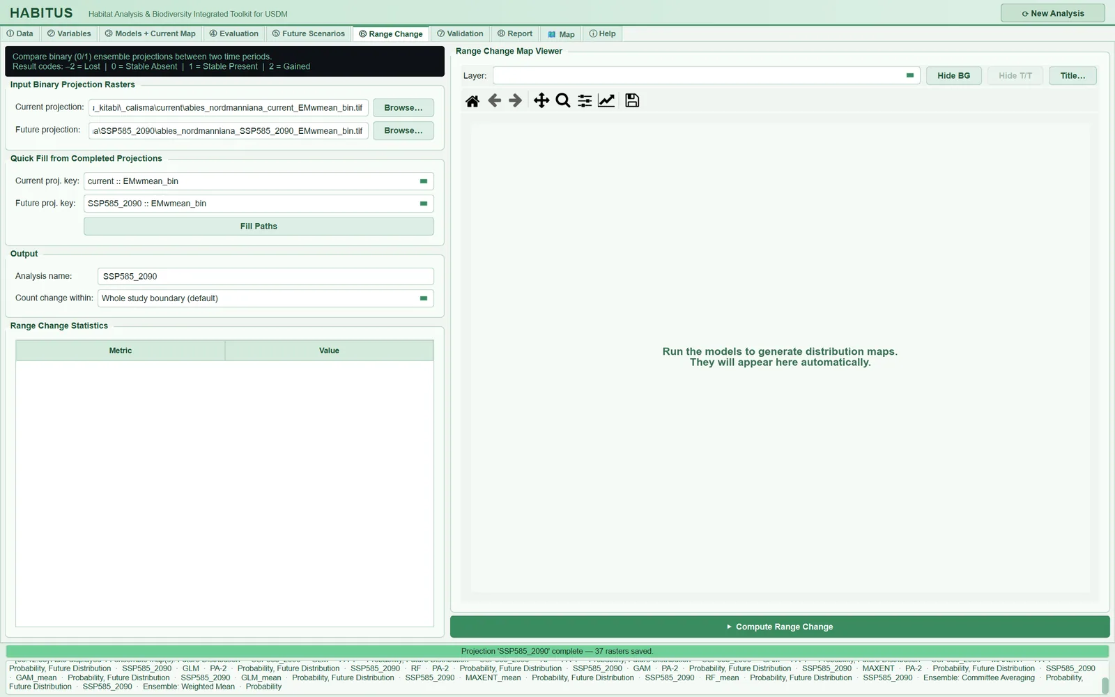
| Area | Name in the UI | Described in |
|---|---|---|
| Information strip | (untitled) | §9.1, §9.7 |
| File selection | Input Binary Projection Rasters |
§9.3 |
| Quick fill | Quick Fill from Completed Projections |
§9.4 |
| Output and extent | Output |
§9.5, §9.6 |
| Statistics table | Range Change Statistics |
§9.8 |
| Map | Range Change Map Viewer (right pane) |
§9.9 |
9.3 Selecting the binary maps (Input Binary Projection Rasters)
| Name in the UI | What it does | Default | Range / options | Code |
|---|---|---|---|---|
Current projection: + Browse… |
Path of the baseline (current) binary map | empty | .tif .tiff .img .asc |
tabs/tab_range.py:42-46, :167-173 |
Future projection: + Browse… |
Path of the (future) binary map to be compared | empty | same | tabs/tab_range.py:48-52 |
- What it does. These two fields are the only input to the computation; the quick-fill lists only fill these fields. In the computation, 1 counts as "present" and 0 as "absent"; other values (e.g. a probability of 0.37) fall into no class (
sdm_core.py:8292-8296). - When and how to set it. The two maps must have been produced with the same method: the same ensemble rule (
EMwmean_binwithEMwmean_bin), the same set of algorithms, the same threshold rule and the same clamping/mask choice. The difference between two maps produced with different methods also carries the effect of the methodological difference, not only of climate change. - Effect on results. Which map is selected is the decision that affects the result most (§9.10).
- Caution. Whether the file selected with
Browse…is binary is not checked; if a_prob.tifis selected by mistake, most cells fall into no class and the counts become meaningless. If both fields are empty, the messagePlease specify both current and future binary rasters.appears (tabs/tab_range.py:200-202).
9.4 Quick fill (Quick Fill from Completed Projections)
| Name in the UI | What it does | Default | Range / options | Code |
|---|---|---|---|---|
Current proj. key: |
Selects the current map from the binary maps in the session | — select — |
<scenario> :: <layer>_bin |
tabs/tab_range.py:62, :128-142 |
Future proj. key: |
Selects the future map from the same list | — select — |
same | tabs/tab_range.py:63 |
Fill Paths |
Writes the file paths of the selected keys into the fields above | — | — | tabs/tab_range.py:64-66, :144-165 |
- What it does. The lists are built from the layers whose names contain
_binamong all projections produced in the session (currentin ③ and every scenario in ⑤) (tabs/tab_range.py:130-131): single models (GLM_PA1_bin), algorithm means (GLM_mean_bin) and ensembles (EMwmean_bin,EMca_bin). The list is refreshed every time the tab is opened; if it has not changed, the user's selection is kept. - When and how to set it. In the example run,
current :: EMwmean_binandSSP585_2090 :: EMwmean_binwere selected andFill Pathswas pressed. Selecting from the list has two advantages overBrowse…: there are no path errors, and the NT1 surface needed for the extrapolation share is found with certainty (§9.6.3). In addition, the multi-species batch run (⑧) repeats the key selected from the list, whereas a path chosen by hand points only to that species' file (tabs/tab_range.py:206-211). - Caution. If
Fill Pathsis pressed while one of the lists is at— select —, the messageFill Paths takes the paths from the lists above. Choose the … binary map in the list first.appears; if the lists are empty, running ③ and ⑤ or usingBrowseis suggested (tabs/tab_range.py:154-165).
9.5 Analysis name (Output · Analysis name)
| Name in the UI | What it does | Default | Range / options | Code |
|---|---|---|---|---|
Analysis name: |
Name of the output file and key of the result in the session | SRC_current_future |
free text | tabs/tab_range.py:76-77, :216, :267 |
The output is written as <output folder>\<species>_<analysis name>_SRC.tif (tabs/tab_range.py:213-216). A second run with the same name overwrites both the file and the result in the session; the report opens a separate subsection for each name. If several scenarios are being compared, name the analysis after the scenario (SSP585_2090 in the example run).
9.6 Extent within which change is counted (Count change within)
| Name in the UI | What it does | Default | Range / options | Code |
|---|---|---|---|---|
Count change within: |
Extent of the headline counts and of the map | Whole study boundary (default) |
Whole study boundary (default) / Accessible area / Accessible area without extrapolation |
tabs/tab_range.py:80-94, sdm_core.py:8179-8184 |
9.6.1 The three extents
- What it does. The selected extent determines the numbers in the upper rows of the table and which cells are coded on the map (
sdm_core.py:8318-8322): Whole study boundary (default): every cell that is valid in both maps.Accessible area: only cells within the accessible area (Min ① Data, the area the species can reach).Accessible area without extrapolation: cells within the accessible area and with ExDet NT1 ≥ 0 in the future scenario (Mesgaran et al. 2014), that is, cells where no variable goes outside its training range (sdm_core.py:8308-8311).
Whichever is selected, if the inputs are available the net change of the other extents is also added to the table as separate rows (tabs/tab_range.py:285-288).
- When and how to set it. If the study boundary is much wider than the area the species can reach, most of the predicted change can accumulate in cells that are near no record and outside the training range (the tooltip text says this, tabs/tab_range.py:85-93). The concept of the accessible area rests on the BAM framework of Barve et al. (2011). For the main number to be reported, Accessible area without extrapolation is the most defensible; the whole study boundary is given alongside it for comparison.
- Effect on results. In the example run (EMwmean_bin) the net change is −46.13 percent over the whole boundary, −30.25 in the accessible area and −16.57 in the accessible area without extrapolation. Depending on the extent, the same two maps give results ranging from "shrinking by half" to "shrinking by one sixth".
- Caution. If there is no accessible area, the second and third options stop with the message No accessible area is available for this run, so change cannot be counted within it. …; if the NT1 surface cannot be found, the third option stops with the message No ExDet NT1 surface was found next to the future map, … (tabs/tab_range.py:224-239).
9.6.2 Where accessible_area.tif comes from
If an accessible-area method (buffer around records, convex hull or user polygon) has been selected in ① Data, this mask is written during data preparation as a 0/1 GeoTIFF on the training grid to the output folder under the name accessible_area.tif (tabs/tab_data.py:1536-1548, sdm_spatial.py:1065-1075). The mask is built from the presence records remaining after thinning (sdm_core.py:2971-2974). In the example run a 200 km buffer around the records was used and the mask covered 40.0% of the raster extent. If no accessible area was selected (buffer 0 km), the file is not written.
9.6.3 Where the NT1 surface comes from
⑤ writes <species>_<scenario>_NT1.tif for every projection (§8.9). ⑥ looks up the path of the future map in the projection records of the session and takes the NT1 file of the scenario it finds; if it finds none, it uses the file ending in _NT1.tif in the same folder as the future map if there is exactly one such file (tabs/tab_range.py:175-193). If the future map was selected from another folder with Browse…, or if the folder contains more than one NT1 file, NT1 cannot be found.
Note: The extrapolation criterion is only the NT1 of the future scenario. The current map may also contain extrapolated cells (23.4% of the current map in the example run); these are not additionally excluded in this extent.
9.7 Result codes and writing of the map
For each cell, and only in cells that are not nodata in both maps (valid), the following codes are written (sdm_core.py:8292-8296, :8319-8322):
| Code | Name | Condition | Colour (viewer) |
|---|---|---|---|
| −2 | Lost | present now, absent in the future | red |
| 0 | Stable Absent | absent now, absent in the future | light grey |
| 1 | Stable Present | present now, present in the future | light turquoise |
| 2 | Gained | absent now, present in the future | green |
Cells outside the selected extent and cells that are nodata in either map remain nodata. If the future map is not on the grid of the current map, it is first aligned by position using the nearest-neighbour method (because it is a binary map; sdm_core.py:8242-8277); the accessible area and NT1 are brought to the current grid in the same way. If alignment was done, a warning is written to the log and the job ends with the message Range change complete; the future raster was not on the current grid and was realigned by position (see log). (tabs/tab_range.py:311-318). The computation is done in row strips according to a memory budget (64 MB; sdm_core.py:8164-8177); the result is identical to a single-pass computation.
9.8 Statistics table (Range Change Statistics)
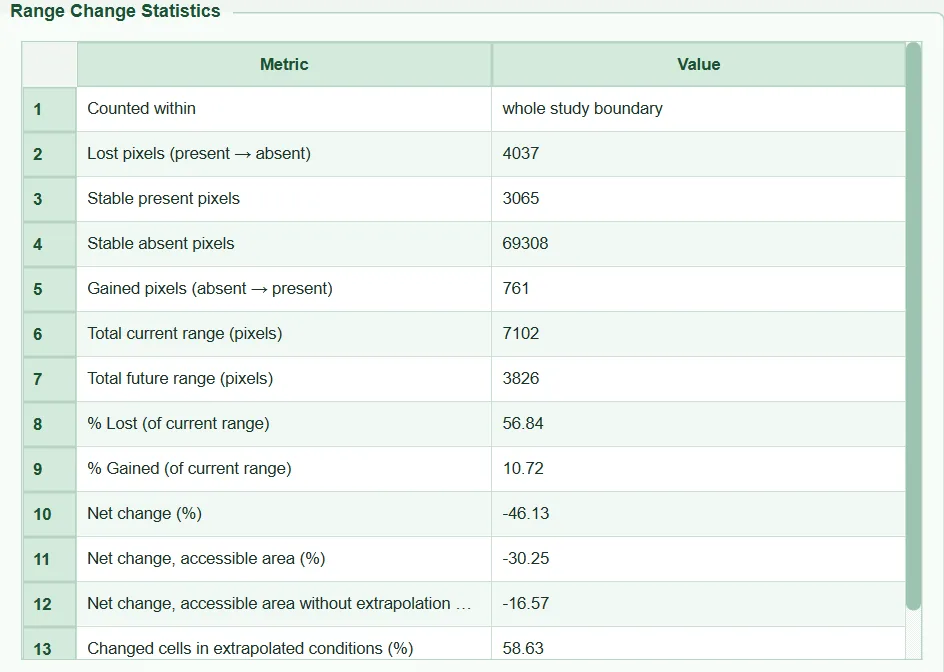
All numbers are cell counts; they are not converted to area units (km²). In the formulas L is the number of lost cells, G gained, S_1 stable present and S_0 stable absent; C=L+S_1 is the current range and F=G+S_1 the future range (sdm_core.py:8187-8193, :8312-8317).
| Row (name in the UI) | Definition | Example run |
|---|---|---|
Counted within |
Name of the selected extent | whole study boundary |
Lost pixels (present → absent) |
L | 4037 |
Stable present pixels |
S_1 | 3065 |
Stable absent pixels |
S_0 | 69308 |
Gained pixels (absent → present) |
G | 761 |
Total current range (pixels) |
C = L + S_1 | 7102 |
Total future range (pixels) |
F = G + S_1 | 3826 |
% Lost (of current range) |
100\,L/C | 56.84 |
% Gained (of current range) |
100\,G/C | 10.72 |
Net change (%) |
100\,(F-C)/C = \%G - \%L | −46.13 |
Net change, accessible area (%) |
same formula, within the accessible area | −30.25 |
Net change, accessible area without extrapolation (%) |
same formula, accessible area ∩ NT1 ≥ 0 | −16.57 |
Changed cells in extrapolated conditions (%) |
100 \times (changed cells with NT1 < 0) / (all changed cells), changed = L+G | 58.63 |
The denominator of the percentages is always the current range (C); if C=0 the denominator is taken as 1 (max(tc, 1)). The gain percentage can therefore exceed 100.
9.8.1 Net change of the other extents
- What it does. The headline numbers are given for the selected extent; if the accessible-area file exists, the row
Net change, accessible area (%)is added automatically, and if NT1 also exists, the rowNet change, accessible area without extrapolation (%)(sdm_core.py:8330-8340). The selected extent's own row is not repeated. - Effect on results. From a single table the reader sees how sensitive the change is to the extent. In the example run there is a difference of about 30 percentage points between the three values.
9.8.2 Extrapolated share of change and the 25% warning
- What it does.
Changed cells in extrapolated conditions (%)tells how many of the lost or gained cells are in places where at least one variable is outside its training range in the future scenario (NT1 < 0) (sdm_core.py:8299-8304,:8341-8343). This share is computed, independently of the selected extent, over all cells that are valid in both maps. - Effect on results. If the share is 25% or above,
WARNING: x% of the cells that change lie in conditions outside the calibration range (ExDet NT1 < 0); treat the change there as extrapolation.is written to the log (tabs/tab_range.py:297-305); a note with the same meaning also appears in the report (§11.5.9). In the example run the share is 58.63%: more than half of the change is in conditions the model has never seen. - Caution. This row appears only when NT1 is found; it does not appear for a future map selected from another folder with
Browse….
9.9 Map
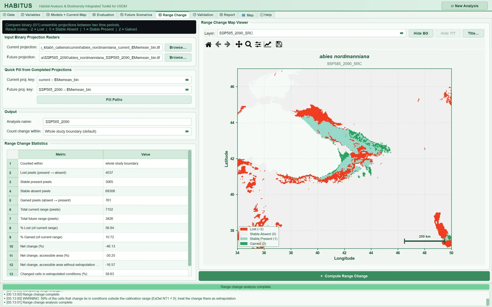
When the job finishes, the <analysis name>_SRC layer is loaded into the viewer with the range_change style (tabs/tab_range.py:307-309). The colours are fixed: red #f03b20 (−2), light grey #f0f0f0 (0), light turquoise #99d8c9 (1), green #2ca25f (2) (map_widget.py:142-146). The viewer controls and publication output are described in Chapter 12. In the example map, losses are concentrated on the low-lying and western margins of the species' current range and gains at the eastern end; the scattered patches of loss in the south and north-east of the study area lie outside the accessible area.
9.10 Which ensemble map should be chosen: EMwmean_bin or EMca_bin?
The two ensemble binary maps are thresholded with different rules (sdm_core.py:6423-6446):
EMwmean_bin: the weighted mean probability map is cut at a threshold that is the mean of the members' own thresholds with the same weights.EMca_bin: the committee average, that is, the proportion of replicates voting "present"; it is cut at 0.5 (majority vote).
For the same current/future pair of the example run, over the whole study boundary (script: sekil/_betik/09_alan_degisimi_karsilastirma.py, using the program's RangeChangeAnalyzer.compute function; "mean" is the binary map of the algorithm mean <ALG>_mean_bin, ranges are cell counts, "access." accessible area, "extrap." extrapolation):
| Binary map | Current | Future | % Lost | % Gained | Net, boundary | Net, access. | Net, no extrap. | Extrap. change |
|---|---|---|---|---|---|---|---|---|
| EMwmean | 7102 | 3826 | 56.84 | 10.72 | −46.13 | −30.25 | −16.57 | 58.6% |
| EMca | 7222 | 3161 | 65.12 | 8.89 | −56.23 | −45.38 | −25.05 | 60.2% |
| GLM mean | 5764 | 1953 | 67.52 | 1.41 | −66.12 | −62.99 | −45.69 | 43.0% |
| GAM mean | 10077 | 4194 | 72.58 | 14.20 | −58.38 | −41.24 | −28.68 | 68.4% |
| MaxEnt mean | 9673 | 3856 | 68.58 | 8.45 | −60.14 | −43.56 | −15.74 | 61.3% |
| RF mean | 7774 | 8264 | 58.01 | 64.32 | +6.30 | +20.58 | −6.41 | 78.6% |
- Effect on results. Changing the ensemble rule alone shifted the net change by 10 points (−46 versus −56). The difference between algorithms is much larger: RF predicts expansion (+6), GLM severe contraction (−66). 78.6% of RF's gains are in extrapolated conditions; because tree-based methods stay constant at the last value outside the range, they can leave large areas that move outside the range in the future as "suitable".
- When and how to set it. For the main result, the map of the rule selected as the ensemble criterion in ③ is used and its name is stated in the methods. If the results of both ensemble rules and of the algorithm means are given in a supplementary table, the reader sees the source of the uncertainty. For this comparison, each map is run with a separate
Analysis name.
9.11 Dispersal assumption
- What it does. The program counts gained cells wherever they are: the species is assumed to be able to reach every cell that becomes suitable in the future (unlimited dispersal). Losses are the same under both assumptions.
- When and how to set it. For slowly spreading species such as trees, the no dispersal assumption should also be reported (Thuiller et al. 2005). In this case the future range consists only of stable present cells: F_{ ext{nd}}=S_1 (future range with no dispersal), and the net change is 100\,(S_1-C)/C = -\%L. In the example run (
EMwmean_bin, whole boundary) this means −56.84 instead of −46.13. The program does not write this number separately; the% Lostrow of the table with a minus sign is the no-dispersal net change. - Caution. The accessible-area extent behaves partly like a dispersal limit: gains outside the area are not counted. However, because the accessible area is built from current records, cells that lie inside this area but that the species could not reach within a century are still counted. There is no option that applies a specific dispersal rate (km/year).
9.12 Outputs and what passes to the next step
<output folder>\<species>_<analysis name>_SRC.tif: float32, codes −2/0/1/2, nodata that of the current map (otherwise −9999).state["range_results"][<analysis name>] = (statistics, file path): the ⑧ report reads this record; grid warnings enter the processing notes of the report (tabs/tab_report.py:1993-1998).run_log[<analysis name>]: keys, paths and extent; the multi-species batch run repeats this record (tabs/tab_range.py:206-211,:240).
9.13 Expert questions
Q1. Is the computation the same as biomod2's BIOMOD_RangeSize function?
Answer: The coding follows the same logic (−2 loss, 0 stable absent, 1 stable present, 2 gain) and the percentages are divided by the current range (sdm_core.py:8187-8193). The difference lies in the additional extents: biomod2 counts only over the whole of the maps supplied; HABITUS additionally gives the net change for the accessible area and for the accessible area without extrapolation, and the extrapolated share of the change (sdm_core.py:8297-8343). The results are cell counts; for km² they must be multiplied by the cell area, and in geographic coordinates the cell area varies with latitude; the program does not perform this conversion.
Q2. Why is net change equal to "% Gained − % Lost"? Answer: F-C=(G+S_1)-(L+S_1)=G-L; since both are divided by C, \%Net=\%G-\%L. Example: 10.72 − 56.84 = −46.12 (−46.13 with the rounding difference). This can be used to check the internal consistency of the table.
Q3. Why do cells outside the accessible area not enter the computation at all; shouldn't they be counted as losses?
Answer: When Accessible area is selected, cells outside the mask are counted in none of the four classes and become nodata on the map (sdm_core.py:8312-8322). The logic is this: in a cell the species cannot currently reach, a "present" prediction shows potential suitability, not a realised distribution; a "loss" in these cells is not the loss of an observed range (Barve et al. 2011). The count over the whole boundary is always made; if the main extent is another option, it is added to the table as the row Net change, whole study boundary (%) (sdm_core.py:8330-8340, tabs/tab_range.py:285-288). Only the net change is added; for the loss and gain counts over the whole boundary, the analysis must be run separately with Whole study boundary.
Q4. Why is "without extrapolation" defined only by the future NT1?
Answer: As NT1 the code uses the surface written by ⑤ for the future scenario (tabs/tab_range.py:175-193, sdm_core.py:8299-8311). Extrapolated cells in the current map are not additionally excluded. A user who wants to exclude the out-of-range part of the current map as well must combine current\…_NT1.tif with the future NT1 outside the program and mask with it; the program has no option for this.
Q5. Is NT2 (novel combinations) used in the change computation?
Answer: No; only NT1 < 0 is excluded (sdm_core.py:8304, :8310-8311). In the example run, cells with NT2 > 1 make up only 0.3% of the future scenario, so the effect is small. In a study where this share is high, the NT2 surface can be used as an additional mask outside the program.
Q6. Is the result reliable if the future map is on a different grid?
Answer: The future map is aligned by position to the grid of the current map: with the same cell size, a whole-cell offset is shifted without interpolation, otherwise it is resampled with nearest neighbour (sdm_core.py:8242-8277, sdm_grid.py:244-280). The alignment is written to the log and to the processing notes of the report. Because the maps produced in ⑤ are already on the training grid, no alignment is needed in normal use.
Q7. Why does the result change with a future map that has the MESS < 0 mask turned on?
Answer: Only cells valid in both maps are counted (sdm_core.py:8292). Masked future cells drop out of the computation; the area that is "present" today in these cells also drops out of C. The result resembles the "Accessible area without extrapolation" option but is not the same: that option additionally restricts to the accessible area and masks the count, not the map.
Q8. How does the choice of threshold affect range change?
Answer: The binary maps are produced with the threshold rule in ③ (default max TSS), and the same threshold is used for both periods (sdm_core.py:7908). As the threshold falls, the "present" area grows in both maps; because the percentages are divided by the current range, the relative change can move in different directions depending on the threshold. In the example run, the net change differs by 10 points between EMwmean_bin and EMca_bin, which differ only in the thresholding rule (§9.10). Threshold sensitivity is tested by rebuilding with a different threshold rule in ③ and repeating ⑥.
Q9. Does a cell being "present" mean that the species will be there? Answer: No. The binary map shows the cells where the suitability value exceeds the threshold; in a presence–pseudo-absence model this means "climatically suitable". Biotic interactions, land use and dispersal limits are not in the model. Gained cells can be counted as new range only under the unlimited dispersal assumption (§9.11).
Q10. Is the result reproducible?
Answer: The computation has no random component; the same two maps give the same count. The selected extent, analysis name and input paths are written to run_log and the results to state["range_results"]; the report contains the table and the map for each analysis. The comparison table in this chapter can be reproduced with sekil/_betik/09_alan_degisimi_karsilastirma.py, which calls the program's own function.
9.14 Common mistakes and pitfalls
- Comparing two maps produced with different methods. If
EMwmean_binis selected for the present andEMca_binfor the future, part of the change comes from the method. - Selecting a probability map with
Browse…. The program does not warn; cells that fall into no class are not counted. - Reporting the whole-boundary result as the only result. In the example run the whole boundary gives −46 and the accessible area without extrapolation −17 percent; which one is reported should be stated explicitly.
- Not stating the dispersal assumption. The net change in the table assumes unlimited dispersal; the no-dispersal value is the
% Lostrow with a minus sign. - Ignoring the extrapolated share of changed cells. A share above 25% says that an important part of the result rests on conditions the model has never seen.
- Taking the number of cells for area. The table counts cells; for km² multiply by the cell area (on a geographic grid it varies with latitude).
- A future map selected from another folder. NT1 cannot be found; the extrapolation share row and the third extent cannot be used.
9.15 References
Barve, N., Barve, V., Jiménez-Valverde, A., Lira-Noriega, A., Maher, S.P., Peterson, A.T., Soberón, J., Villalobos, F., 2011. The crucial role of the accessible area in ecological niche modeling and species distribution modeling. Ecological Modelling 222, 1810–1819. https://doi.org/10.1016/j.ecolmodel.2011.02.011
Mesgaran, M.B., Cousens, R.D., Webber, B.L., 2014. Here be dragons: a tool for quantifying novelty due to covariate range and correlation change when projecting species distribution models. Diversity and Distributions 20, 1147–1159. https://doi.org/10.1111/ddi.12209
Thuiller, W., Lafourcade, B., Engler, R., Araújo, M.B., 2009. BIOMOD – a platform for ensemble forecasting of species distributions. Ecography 32, 369–373. https://doi.org/10.1111/j.1600-0587.2008.05742.x
Thuiller, W., Lavorel, S., Araújo, M.B., Sykes, M.T., Prentice, I.C., 2005. Climate change threats to plant diversity in Europe. Proceedings of the National Academy of Sciences 102, 8245–8250. https://doi.org/10.1073/pnas.0409902102