2. Data I: records, layers and study boundary (① Data)
Tab: ① Data · Code: tabs/tab_data.py (UI), sdm_inputs.py (CSV reading), sdm_mask.py (folder scanning, clipping to the boundary), sdm_core.py DataFormatter (loading and record filtering)
2.1 What this tab does
① Data is the first and mandatory step of the workflow. It reads the species records (presence points), the predictor raster layers and an optional study boundary; it filters the records; it then generates the pseudo-absence sets for the machine learning models, the background points for MaxEnt and a separate background sample for ENFA. This chapter covers the "data" half of the tab: the record file, the layers, the boundary, the seed, the output folder and every operation that Load Data performs on the records. The background, pseudo-absence, accessible area and thinning settings are in Chapter 3.
- Input: an occurrence CSV (species name, longitude, latitude), at least one continuous raster, optional categorical rasters and a boundary layer.
- Output: the in-memory
DataFormatterobject (predictor arrays, filtered presences, pseudo-absence sets, backgrounds), counts written to the log and to the run record (habitus_run_config.json); if a boundary is given, clipped layers (masked_inputs/current/); if an accessible area is defined,accessible_area.tif. - Lock order: when the step finishes successfully, the ② Variables tab is unlocked and the program switches to it (
tabs/tab_data.py:1759-1760). If ① is run again, all results of the later tabs are reset (tabs/tab_data.py:1396-1397).
2.2 Screen layout
The tab consists of two columns (tabs/tab_data.py:78-82). The left column holds the record file, the raster lists and the study boundary; the right column holds the background/pseudo-absence settings, reproducibility and the output folder. At the bottom is the green button that starts the whole step, with the progress bar and the session log below it.
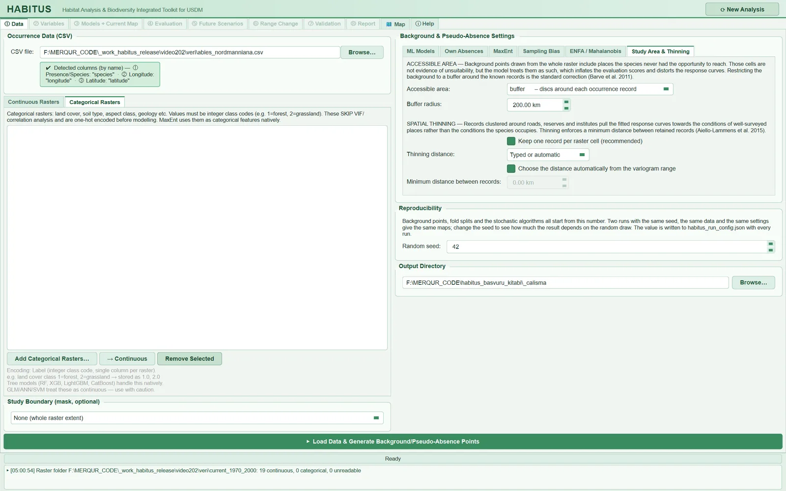
| Region | Name in the UI | In this book |
|---|---|---|
| Top left | Occurrence Data (CSV) |
§2.3 |
| Middle left | Continuous Rasters, Categorical Rasters |
§2.4 |
| Bottom left | Study Boundary (mask, optional) |
§2.5 |
| Top right | Background & Pseudo-Absence Settings (6 sub-tabs) |
Chapter 3 |
| Middle right | Reproducibility |
§2.6 |
| Bottom right | Output Directory |
§2.7 |
| Bottom bar | Load Data & Generate Background/Pseudo-Absence Points |
§2.8, §2.9 |
2.3 Species records: Occurrence Data (CSV)
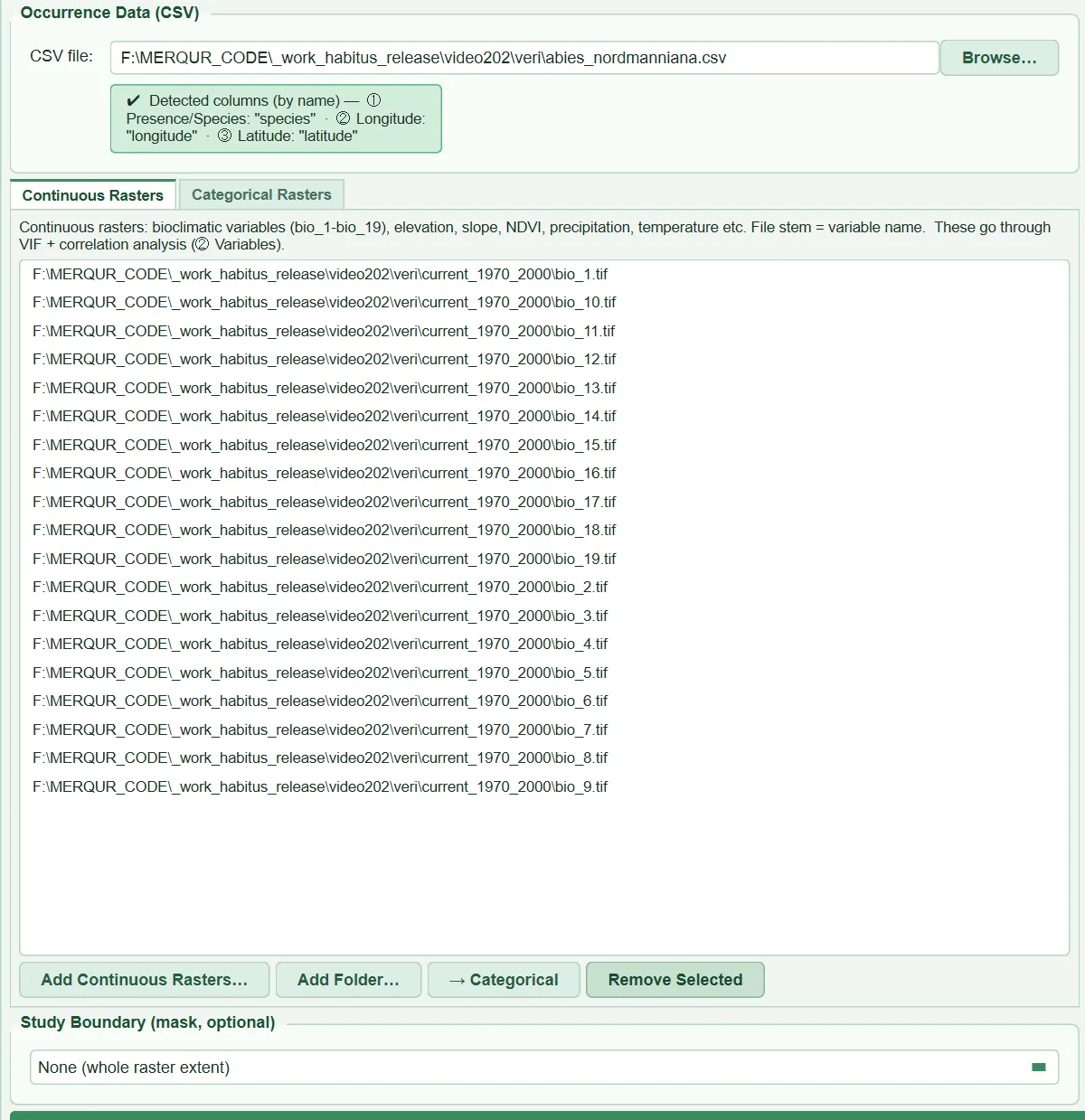
This group reads the table holding the coordinates of the places where the species was observed. When a file is selected, the program inspects the first rows, identifies the columns, states in a green information box which column will be used as what and, if the file contains more than one species, opens a species list.
| Name in the UI | What it does | Default | Range / options | Code |
|---|---|---|---|---|
CSV file: + Browse… |
Selects the record table; on selection scans the columns and species and suggests an output folder | empty | .csv, .tsv, .txt |
tabs/tab_data.py:92-96, 972-979 |
| Information box | Shows the detected species, longitude and latitude columns and the columns that will be ignored | — | — | tabs/tab_data.py:99-108, 1008-1023 |
Species: list |
In a multi-species file, one checkbox per species (with its record count) | all ticked | All / None |
tabs/tab_data.py:112-149, 1045-1072 |
Analyse now: |
Selects the species for which the ①–⑧ workflow will now run | first ticked species | ticked species | tabs/tab_data.py:132-140, 1085-1095 |
2.3.1 File format, delimiter and decimal mark
- What it does. The program reads every CSV with the same routine (
sdm_inputs.py:20-65). The first 50 non-empty lines are taken from the first 64 KB of the file; the count of commas, semicolons and tabs is computed for each line, and the character that occurs the same number of times in most lines is taken as the delimiter. If the delimiter is a semicolon or a tab and the body contains numbers of the form36,52while there is no dot decimal at all, the decimal mark is taken to be the comma. The file is read as UTF-8; a leading byte order mark (BOM) is discarded. - When and how to set it. There is no setting; a
;-delimited, comma-decimal file saved by a spreadsheet with a Turkish, German or Spanish regional setting is read as is. The safest format is still comma delimiter and dot decimal. - Effect on results. A wrongly detected delimiter collapses the whole table into a single column; in that case the program issues the warning "CSV has only 1 column(s)" and no coordinates are read.
- Caution. In a comma-delimited file, if coordinates are written with a comma inside quotes, such as
"36,52", the decimal comma is not detected (detection is done only for;and tab) and the coordinate column remains text. Any coordinate cell that cannot be converted to a number stops the run with the row number: "column '…' holds non-numeric coordinates in N row(s) (row 5: '36°31′'…)" (sdm_inputs.py:100-123). Empty coordinate cells, however, do not stop it; those records are dropped with the reason "missing coordinate" and a warning is written (sdm_core.py:2944-2953). A non-UTF-8 file is rejected with the message "Re-save it as 'CSV UTF-8'" (sdm_inputs.py:90-93).
2.3.2 Column detection (by name, by position, GBIF)
- What it does.
occurrence_columnsfirst looks at the names (sdm_inputs.py:128-166). Case-insensitively,longitude, decimallongitude, lon, long, lng, xare searched for longitude andlatitude, decimallatitude, lat, yfor latitude. If both are found, the species column is the first of the namesspecies, scientificname, acceptedscientificname, verbatimscientificname, taxon; if none of these exists, the first non-coordinate column is taken. If the coordinate names cannot be found, the first three columns are read by position: ① species, ② longitude, ③ latitude. The suffix "(by name)" in the information box shows that the columns were found by name. If the file has more than three columns, the extra ones are ignored and an information window lists them one by one ("Extra Columns Detected",tabs/tab_data.py:1030-1041). - When and how to set it. A Darwin Core table downloaded from GBIF (
gbifID, …, species, …, decimalLongitude, decimalLatitude) can be used without editing. In your own table, naming the columnsspecies, longitude, latitudeis the clearest route; there is no separate field in the UI for selecting columns. - Effect on results. Swapping longitude and latitude throws most records outside the raster. The program tries to detect this situation (§2.8.6).
- Caution. When no names are found, the order is strictly "species, longitude, latitude"; a file in the order "species, latitude, longitude" is read the wrong way round. If only columns named
xandyexist, they are also taken as coordinates. The initial information text in the UI ("The first 3 columns will always be used") appears before a file is selected; once a file is selected, the columns actually used are written, and this is what counts.
2.3.3 Multi-species file and Analyse now
- What it does. If the species column holds more than one name, the
Species:row opens; each species is listed as a checkbox with its record count (tabs/tab_data.py:1045-1072). If all values in the column are numbers (e.g. a 0/1 presence code), they are not treated as species names and the list does not open. TheAnalyse now:box selects one of the ticked species. WhenLoad Datais pressed, only that species' records are taken, written asoccurrences_used.csvto a subfolder named after the species inside the output folder, and the workflow continues with this file (tabs/tab_data.py:1500-1506). - When and how to set it. To model many species with the same settings: first complete ①–⑧ for one species, then
Run Selected Speciesin ⑧ Report applies the same settings to the other ticked species (Chapter 11). - Effect on results. Each species is modelled separately, with its own records; no information is shared between species. Subfolder names are made file-system safe and de-duplicated case-insensitively ("Quercus robur" and "quercus robur" go to separate folders;
tabs/tab_data.py:34-60). - Caution. If no species is ticked, the run stops with the message "The occurrence file holds several species. Tick at least one and choose it under 'Analyse now'." (
tabs/tab_data.py:1373-1378). Leading and trailing spaces in species names are trimmed; "Abies nordmanniana" and "Abies nordmanniana" (two spaces) are still counted as two different species.
2.3.4 Species name and suggested output folder
The species name used in reports and file names is determined as follows (sdm_core.py:1566-1593): if the first column is neither a coordinate nor the species column and is not numeric, the most frequent text in it; otherwise the most frequent text in the species column; failing that, the name of the CSV file (underscores and hyphens converted to spaces). In the sample run the name is "abies nordmanniana". If Output Directory is empty, a folder Documents/HABITUS/<species>_YYYYMMDD_HHMMSS is created as soon as the file is selected and written into the field (tabs/tab_data.py:1125-1160, main_dialog.py:832-853); for a multi-species file the folder name is taken from the CSV name.
2.4 Predictor layers: Continuous Rasters and Categorical Rasters
Predictors are kept in two separate lists. Continuous layers are measured quantities: temperature, precipitation, elevation, slope, NDVI. Categorical layers are class codes: land cover, soil type, geology. This distinction affects every subsequent step: continuous layers enter the VIF and correlation analysis in ② Variables, while categorical layers are excluded from that analysis and are passed to the models as classes.
| Name in the UI | What it does | Default | Range / options | Code |
|---|---|---|---|---|
Add Continuous Rasters… |
Adds the selected files to the continuous list (the same path is not added twice) | — | .tif .tiff .asc .img .nc .vrt |
tabs/tab_data.py:911-912, 1183-1191 |
Add Folder… |
Reads all rasters in the folder and classifies each as continuous/categorical | — | folder | tabs/tab_data.py:913-919, 1205-1290 |
→ Categorical / → Continuous |
Moves the selected files to the other list | — | — | tabs/tab_data.py:920-922, 948-950, 1197-1203 |
Remove Selected |
Removes the selected files from the list | — | — | tabs/tab_data.py:923-924, 1193-1195 |
Add Categorical Rasters… |
Adds the selected files to the categorical list | — | same extensions | tabs/tab_data.py:946-947 |
| Encoding note | States that the categorical encoding is label (integer class code) | label | label only | tabs/tab_data.py:959-968, sdm_core.py:1428-1440 |
2.4.1 Adding files individually and variable names
- What it does. The name of each file without its extension becomes the variable name. The name is cleaned by converting spaces, parentheses, hyphens and dots to underscores:
bio_ (1)→bio_1,tr-elev→tr_elev(sdm_core.py:166-186). Whatever order the layers were added to the list in, the program sorts the variables in "natural" order (bio_2 < bio_3 < bio_12;sdm_core.py:189-200,1617-1620); thus the results do not depend on the order of addition. - When and how to set it. Because layers are matched by name in future scenarios (⑤), current and future files must have the same names (
bio_1.tif↔bio_1.tif). - Effect on results. Only the first band of each layer is read (
sdm_core.py:1608); the other bands of a multi-band GeoTIFF or NetCDF are not used. Continuous layers are held in memory as float32 if the source type can be carried losslessly, otherwise as float64 (sdm_core.py:1367-1379); values are preserved bit for bit, and all computations are done in float64. - Caution. The layer's NoData value must be defined in the file; if it is not, sea or empty cells (e.g. -3.4e38) are taken as real values. Two files that give the same name after cleaning (
bio 1.tifandbio_1.tif) are not checked when no boundary is used; the one read later replaces the earlier one. When a boundary is used, two files with the same name give an error: "Two predictor rasters have the same name" (sdm_mask.py:337-345).
2.4.2 Add Folder…: continuous/categorical classification and its rationale
- What it does.
scan_raster_foldersorts the.tif .tiff .asc .img .nc .vrtfiles in the folder by name and classifies each withclassify_raster(sdm_mask.py:54-141). The rules, in order, are:- A file whose name looks like a bioclimatic layer (
bio1,bio_12,wc2.1_30s_bio_5) and which carries no colour table is taken as continuous without reading its values (so the gigabytes of text of a 30 arc-second global.ascare not read). - Other files are read decimated: downsampled by nearest neighbour so that the long side is at most about 1000 cells.
- If there are no valid cells, the file is left continuous and flagged as suspicious.
- If there is a colour table (palette), categorical.
- If there are decimal values, continuous.
- If all values are integers and the number of distinct values is at most 30 (
MAX_CATEGORICAL_CLASSES), categorical; if there are at least 12 distinct values and the name contains no word suggesting classes, or the name suggests a continuous variable (elev,slope,ndvi,temp,prec…), it is flagged as suspicious. - If there are more than 30 distinct integers, continuous; suspicious if the name contains
landcover,soil,geolog,class,zone….
- A file whose name looks like a bioclimatic layer (
- When and how to set it. This is the fastest route for a user who keeps bioclimatic and other layers in one folder. The result window ("Rasters added") lists each file with the letter
N(continuous) orC(categorical) and its rationale; rows marked ⚠ should be checked by hand, and a misclassified file should be moved with→ Categorical/→ Continuous. - Effect on results. In the sample data all 19 files were taken as continuous from their names (log: "19 continuous, 0 categorical, 0 unreadable"). A layer left in the wrong list is misrepresented in the model: a temperature layer left in the categorical list does not enter the VIF analysis and is treated as classes.
- Caution. Ordinal integer scales such as a 1–5 productivity score cannot be distinguished from class codes by their values and are taken as categorical without being flagged (
sdm_mask.py:48-51). Files that cannot be opened are reported with a "✖ … could not be opened" row and are not added to the list.
2.4.3 How categorical layers enter the model
- What it does. Categorical layers are read converted to integer (int32), NoData cells are marked with
-9999, and the class list of each layer is extracted (sdm_core.py:1653-1677). At the sampled points each layer appears as a single column holding the class code itself (label encoding). The code is not used as a number: the first step of the GLM, GLMNET, SVM and ANN pipeline expands each class into a separate 0/1 column (_CatPrep,sdm_core.py:3364-3384); GAM uses a factor term and MaxEnt the categorical feature class; tree methods (RF, GBM, BRT, XGBoost, LightGBM, CatBoost, CART) split on the code; BIOCLIM, Domain, ENFA and Mahalanobis leave categorical layers out (sdm_core.py:1781-1787). - When and how to set it. For genuine class layers such as land cover. For a species with few records, a layer with many classes produces classes with no or very few records in the training data; the program reports these with a "sparse classes" warning (
sdm_core.py:3232-3246) and offers the option of excluding the layer in ② Variables. - Effect on results. Cells where a categorical layer is NoData are removed from all sampling (
_valid_cell_mask,sdm_core.py:2309-2330); a land cover layer with narrower coverage than the continuous layers shrinks the study area. The numbers of records and cells lost for this reason alone are reported to ② Variables (sdm_core.py:3073-3078). - Caution. Decimal values are truncated when converted to integer (2.7 → 2). A file in the categorical list must also be on the same grid as the continuous layers (§2.4.5). At least one continuous layer is mandatory; running with only categorical layers stops with the message "Please add at least one environmental raster." (
tabs/tab_data.py:1368-1369).
2.4.4 Converting large ASCII grids to GeoTIFF
- What it does. If the total size of the
.ascfiles added withAdd Folder…exceeds 200 MB (_ASC_CONVERT_MB), the program offers to convert them once to compressed, tiled (DEFLATE) GeoTIFF copies ("Convert ASCII grids to GeoTIFF?";tabs/tab_data.py:1292-1330,sdm_mask.py:144-178). The copies are written with the same names to ageotiff/subfolder inside the folder, and the paths in the list are replaced with them; the.ascfiles are not touched. A copy that is newer than its source is not regenerated. - When and how to set it. "Yes" is recommended for global
.asclayers: because ASCII text is parsed from scratch at every read, clipping, sampling and projection each take minutes; GeoTIFF is read window by window. - Effect on results. Values and the coordinate system remain the same; only the run time is shortened.
- Caution. The offer appears only when adding by folder; it is not asked for
.ascfiles added individually.
2.4.5 Grid alignment and coordinate system
- What it does. The program reads all layers cell by cell into a single table; therefore, when no boundary is used, every layer must have the same number of rows and columns, cell size, origin and coordinate system as the first layer (the first name in natural order). A difference of 1e-6 units in cell size and origin is tolerated (
sdm_core.py:1683-1744). Each non-matching layer is listed with its name and the difference: "Environmental rasters are not on the same grid. • bio_12: cell size …". - When and how to set it. Layers from different sources should be aligned beforehand (QGIS: Raster > Align Rasters). Alternatively, if a study boundary is given, the program brings the layers to a common grid itself (§2.5.2).
- Effect on results. The coordinate system can be geographic (degrees) or projected (metres). Every distance-based decision (thinning, buffer, minimum distance, block size) is made in kilometres using great-circle (haversine) distance; on a projected grid the coordinates are first converted to longitude/latitude (
sdm_spatial.py:113-141). If the length unit of a projected system cannot be read, the run stops ("The length unit of the raster coordinate system could not be determined";sdm_spatial.py:93-110). - Caution. The coordinates of the occurrence CSV must be in the same coordinate system as the rasters. The program does not reproject the CSV; it converts the coordinates to cells directly with the raster's transform matrix (
sdm_core.py:1763-1765). If a raster in UTM is used with a CSV in degrees, all records fall outside the raster. When the rasters are geographic, a warning is given for coordinates whose latitude exceeds ±90 or whose longitude exceeds ±180 (sdm_inputs.py:179-196). If the cell size at the equator is about 4 km or larger, a resolution warning is written (sdm_core.py:1751-1761); in the sample run (2.5′, about 4.6 km) this warning appeared.
2.5 Study boundary: Study Boundary (mask, optional)
This group clips all rasters with a polygon or with a rectangle in degrees. Global layers can thus be used without being cut beforehand, and every cell outside the boundary becomes NoData.
| Name in the UI | What it does | Default | Range / options | Code |
|---|---|---|---|---|
| Mode box | Selects the type of boundary | None (whole raster extent) |
None (whole raster extent) / Polygon layer (SHP, GPKG, KML, GeoJSON) / Corner coordinates (degrees) |
tabs/tab_data.py:173-181 |
File field + Browse… / Clear |
Polygon layer (visible only in the second mode); selecting a file switches the mode to polygon automatically | empty | .shp .gpkg .geojson .json .kml .gml |
tabs/tab_data.py:161-172, 1332-1339 |
West / South / East / North |
Corners of the rectangle, WGS84 degrees (third mode only) | 25 / 35 / 45 / 43 | longitude −180…180, latitude −90…90; 4 decimals | tabs/tab_data.py:186-197 |
2.5.1 Modes and the scope of clipping
- What it does. When a boundary is given,
Load Datafirst of all clips all continuous and categorical layers (tabs/tab_data.py:1511-1524). Every subsequent step (record filtering, pseudo-absences, background, cross-validation folds, the current map, the future layers in ⑤ and the ⑥ range change) sees only the cells inside the boundary, because a cell that is NoData in one layer is excluded everywhere. Corner coordinates are taken as an EPSG:4326 rectangle and converted to the raster's system if needed (sdm_mask.py:193-201). - When and how to set it. When the model and maps must be restricted to a country, a catchment or a region. The boundary differs from the accessible area described in Chapter 3: the boundary clips all layers and maps; the accessible area only narrows the area from which background and pseudo-absences are drawn, and the map is still produced for the whole boundary.
- Effect on results. Records falling outside the boundary are dropped with the reason "outside raster extent" or "falls on NoData cell". Because the background is drawn only from inside the boundary, narrowing the boundary affects the evaluation scores in a way similar to narrowing the accessible area (Chapter 3).
- Caution. The check "West must be smaller than East and South smaller than North" is performed (
tabs/tab_data.py:1488-1491). In polygon mode, if there is no file, the run stops with the message "The study boundary layer was not found". If the layer has no polygons ("has no polygon features"), if the boundary does not overlap the rasters at all, or if a layer has no values inside the boundary, the run stops and names the layer (sdm_mask.py:213-216,369-383,399-403). If the boundary layer or the rasters do not declare a coordinate system, the two are assumed to be the same and this is written to the report with a warning (sdm_mask.py:228-236).
2.5.2 How clipping is done: single window, common grid, masked_inputs
- What it does.
mask_rasters(sdm_mask.py:304-418) computes, on the first layer of the list, a single window corresponding to the bounding box of the boundary; all layers are written to the grid of this window. A layer with the same cell size and alignment is read through the window (values unchanged); a layer with a different resolution, a shifted origin or another coordinate system is resampled to this grid by nearest neighbour (sdm_mask.py:273-301). Cells outside the polygon are then set to NoData. The clipped copies are written as GeoTIFF with their original names under<output folder>/masked_inputs/current/; the progress bar shows "Rasters clipped to the study boundary: R x C cells.". - When and how to set it. For using together layers that were cut to different extents or downloaded one cell wider (common in GCM sets), the boundary mode is a practical way of aligning them.
- Effect on results. Nearest neighbour produces no new values and preserves class codes; but when a fine-resolution continuous layer is brought down to a coarse grid, the value of a single cell is taken, not the mean. The future layers in ⑤ are clipped to the same grid, so the current and future maps overlap cell by cell.
- Caution. The grid is determined by the first layer of the list (first the continuous, then the categorical list, in order of addition). Putting the layer with the finest resolution first prevents loss of information. For a multi-species file the
masked_inputsfolder is also in the main output folder; the species share the same clipped copies.
2.6 Reproducibility: Reproducibility
| Name in the UI | What it does | Default | Range / options | Code |
|---|---|---|---|---|
Random seed: |
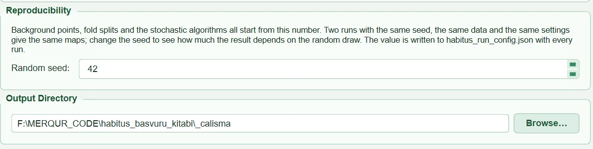
Starting number for all random operations | 42 | 0 – 2147483647 | tabs/tab_data.py:242-249, run_config.py:28 |
2.6.1 Random seed
- What it does. When the data step starts,
set_run_seedseeds NumPy's global generator, Python'srandommodule and thePYTHONHASHSEEDenvironment variable with this number (tabs/tab_data.py:1510,run_config.py:31-50).DataFormatteralso builds its own generator (numpy.random.default_rng(seed)) from this number; pseudo-absences, background draws, the thinning order, the variogram subsample and k-means derive from it (sdm_core.py:1503-1505,2301-2302,2536). Therandom_stateof the models is also given from the same number (Chapter 5). - When and how to set it. In a study to be published, the value is reported; it is written to the
random_seedfield of thehabitus_run_config.jsonfile at every run. To see how much the result depends on the random draws, several different seeds are tried with the same settings. - Effect on results. The same data, the same settings and the same seed are expected to give the same maps. When the seed changes, the pseudo-absence and background points, the folds and the stochastic algorithms change; the fluctuation in the scores and maps shows the sensitivity of the data to these draws.
- Caution.
PYTHONHASHSEEDis set only if it is not already defined (setdefault), and setting it after the Python interpreter has started does not affect hash ordering. Whether multi-threaded libraries (e.g. some gradient boosting implementations) give bit-for-bit identical results on different machines is not guaranteed in the code and has not been tested; reproducibility on the same machine with the same installation is the aim.
2.7 Output folder: Output Directory
| Name in the UI | What it does | Default | Range / options | Code |
|---|---|---|---|---|
Folder field + Browse… |
Folder to which all outputs are written | when a CSV is selected, Documents/HABITUS/<species>_<time> |
any folder | tabs/tab_data.py:253-260, 1125-1160 |
It does not affect the results; if left empty, the run stops with the message "Please specify an output directory.". In a multi-species file each species is written to the <output folder>/<species> subfolder (tabs/tab_data.py:1115-1123); the session log is also moved to this folder at the start of the run, so in a batch run each species' log is in its own folder (tabs/tab_data.py:1398-1408).
2.8 The Load Data button: order of operations and record filtering
The ▶ Load Data & Generate Background/Pseudo-Absence Points button runs the whole step in the background, without freezing the UI (tabs/tab_data.py:1363-1574). The order of operations matters for understanding which record was dropped and why:
- Pre-check: does the CSV exist, is there at least one continuous raster, is the output folder filled in, do the target-group CSV and the bias raster (if given) exist, is the boundary valid.
- If there was a previous data step, all results of the later tabs are reset.
- In a multi-species file, only the records of the selected species are separated into
occurrences_used.csv. - The seed is set (§2.6).
- If a boundary is given, all layers are clipped (§2.5).
load_data: the CSV and the layers are read, the species name is determined, grid alignment is checked (sdm_core.py:1549-1681).generate_pa_datasets: coordinates are converted to numbers, records are filtered (this chapter), thinning and the accessible area are applied, pseudo-absence sets and backgrounds are drawn (Chapter 3), and the collinearity pre-computation is performed (sdm_core.py:2911-3249).- The accessible area is written as
accessible_area.tif; if requested, the MaxEnt background is saved to CSV.
2.8.1 Steps of record filtering
Presence records are filtered in the following order (sdm_core.py:2931-2968, 1824-2037). Every dropped record enters the dropped_points list with its reason; the list appears in the warning window, the log, the report and habitus_run_config.json (points_dropped_by_reason).
| Order | Reason (text in the UI) | Rule | Can it be turned off | Code |
|---|---|---|---|---|
| 1 | missing coordinate |
Longitude or latitude cell is empty | no | sdm_core.py:2944-2953 |
| 2 | duplicate coordinate |
Identical to an earlier record when the coordinates are rounded to 8 decimals | no | sdm_core.py:1844-1856 |
| 3 | outside raster extent |
Cell row/column is outside the grid | no | sdm_core.py:1864-1876 |
| 4 | falls on NoData cell |
NaN in any continuous layer or NoData in any categorical layer | no | sdm_core.py:1878-1905 |
| 5 | same raster cell as another record |
A record earlier in file order exists in the same predictor cell | yes: Keep one record per raster cell |
sdm_core.py:1913-1936 |
| 6 | spatially thinned |
A retained record exists within the thinning distance | yes (Chapter 3) | sdm_core.py:2960-2968 |
2.8.2 Duplicate coordinates, outside the raster and NoData
- What it does. An exactly identical coordinate (up to a rounding difference of about 1 mm) is kept only where it first occurs. Of the remaining records, those falling outside the grid and those falling on a cell with no value in some layer are dropped. Records dropped because of a categorical layer are counted separately (
cat_nodata_loss_presence) and reported to ② Variables. - When and how to set it. These three filters always run; there is no setting.
- Effect on results. At coarse resolution some coastal records may fall on a sea cell and be caught by NoData. The share of dropped records determines the number of presences used and hence the prevalence in Chapter 3.
- Caution. If more than 20% (
LOSS_WARN_FRACTION) of the non-duplicate records fall outside the raster or on NoData, the program swaps longitude and latitude and tries again; if at least half of the records fall inside in the swapped state, it gives the warning "The lon/lat columns are probably swapped", otherwise the warning asking you to check the coordinate system and the columns (sdm_inputs.py:199-221,sdm_core.py:1969-1990). When all records are lost and one layer is NoData at every record inside the extent, the culprit is that layer, not the coordinates; the message names the layer (sdm_core.py:2014-2029).
2.8.3 One record per cell
- What it does. Records falling in the same predictor cell carry the same predictor values; each extra record adds weight to that cell without adding information. With the option on, the first record in file order is kept in each cell and the others are dropped with the reason "same raster cell as another record" (
sdm_core.py:1913-1936). With the option off, these records are still counted and a warning is written (sdm_core.py:1962-1967). The checkbox itself is in the Study Area & Thinning sub-tab (Chapter 3,tabs/tab_data.py:722-731); its default is on. - When and how to set it. It should almost always stay on. Turning it off comes into question only for species with very few records concentrated in a few cells; even then the records repeat the same cell values.
- Effect on results. In the sample run, 405 of the 626 records were dropped because they fell in a cell that already had a record, leaving 221 records (session log). Had it been off, a few intensively observed areas (e.g. hundreds of records in the same valley) would have dominated both the model curves and the cross-validation folds.
- Caution. The rule is applied before thinning. Which record is kept depends on file order; even if the records in the same cell have different coordinates, their predictor values are the same, so there is no difference for the model, but thinning and spatial blocks use the exact location of the record. The external test set (⑦) is exempt from this rule.
2.8.4 At least five presences
- What it does. If at least 5 records (
MIN_PRESENCES,sdm_core.py:1269) do not remain after the filters, the run stops. The message varies with the cause (sdm_core.py:1997-2035): if the loss is due only to the one-per-cell rule, "The N presence record(s) fall in only K predictor cell(s)…"; if there is no loss at all, "Only K usable presence record(s). At least 5 are required…"; if the losses come from outside-raster/NoData, the coordinate system warning. - When and how to set it. It cannot be changed. The threshold rests on the smallest samples in published studies comparing SDM methods (Hernandez et al. 2006; Pearson et al. 2007).
- Effect on results. With 5–24 records the run continues but warnings appear (§2.8.5).
- Caution. This limit is checked before thinning. If fewer than 10 records remain after thinning, only a warning is given ("Thinning at … km leaves only N records";
sdm_core.py:2547-2552); the run does not stop.
2.8.5 Warnings on record count and the record/predictor ratio
- What it does.
_check_sample_size(sdm_core.py:2843-2885) compares the number of presences remaining after thinning (n) with the number of loaded predictors (k: continuous + categorical) and can produce three warnings:- n < 10: "Only N usable presence record(s). No species distribution method produces a trustworthy model at this sample size…"
- n < 25 (
JACKKNIFE_RECOMMENDED_MAX,sdm_spatial.py:594): selecting jackknife validation (leaving out one presence at a time) in ③ Models is recommended (Pearson et al. 2007). - n \geq 10 and n/k < 10: "N presence records for the K predictors loaded (R per predictor)…". The text states that the number of predictors to be kept in ② Variables is the number that really matters and that n records can support about \lfloor n/10 \rfloor predictors.
- When and how to set it. The rule of 10 records per predictor is a common guideline for logistic-type models; flexible learners (RF, boosting, MaxEnt with hinge features) require more (Wisz et al. 2008).
- Effect on results. In the sample run, with 143 records and 19 layers the ratio is 7.5; the message says "143 records allow about 14". When 8 variables are kept in ② Variables (ratio 17.9), the same check is repeated and the warning disappears (
note_selected_predictors,sdm_core.py:2889-2909;tabs/tab_vif.py:1213). - Caution. The warnings do not change the result; they are written to the report as "advisory". The k in this section counts all layers loaded in ① Data; for the number after selection, the message in ② is authoritative.
2.8.6 Messages after the data step
When the step finishes, the following windows appear in order (tabs/tab_data.py:1576-1761):
- "Invalid Occurrence Points Detected": if at least one record was dropped; one heading per reason and a list of coordinates (under the cell and thinning headings the first 15 records, the rest as "… and N more"), ending with "✔ N valid point(s) will be used for modelling." and a CRS reminder. The same text is written to the log.
- "Points worth knowing before you interpret this run": warnings that affect the interpretation of the result (resolution, record/predictor ratio, accessible area, thinning, absence records…). If the only warning is the sampling bias reminder, this window does not open and the warning is written only to the log with the prefix "ADVISORY:".
- "Data ready!" summary: number of presences used/loaded, breakdown of dropped records by reason, the pseudo-absence or true absence row, number of MaxEnt background points, the accessible area and the share it covers, the thinning distance and how it was chosen, the autocorrelation range, prevalence, the note that sampling bias has not been corrected, the seed, and the names of the continuous and categorical variables.
The summary of the sample run, compiled from the session log, is as follows: 626 records loaded; 405 dropped as same cell and 78 by thinning; 143 presences used; 2 sets × 1000 pseudo-absences; 10,000 MaxEnt background points; accessible area buffer, 200 km, 40% of the raster extent; thinning 4.7 km (automatic); autocorrelation range 151.5 km; prevalence 0.125.

2.9 Outputs and what passes to the next step
- In memory (for ② onwards): predictor arrays, variable names (
var_names,cat_var_names), pseudo-absence sets (pa_datasets), MaxEnt and ENFA backgrounds, filtered presences, the autocorrelation range (used as the spatial block size in ③), the collinearity pre-ranking (collinearity_df, the starting table of ② Variables). - On disk:
masked_inputs/current/*.tif(if a boundary is given),occurrences_used.csv(in a multi-species file),accessible_area.tif(if an accessible area is defined; 1 = inside, 0 = outside),background_maxent.csv(if requested), the session loghabitus_<time>.log. - Run record: the
datasection ofhabitus_run_config.jsoncontains the CSV used, the species name, the number of presences used, the breakdown of dropped records by reason, the raster lists, the grid information (raster_grid: reference layer, rows-columns, cell size, km at the equator, CRS) and the prevalence; thestudy_boundarysection contains the boundary, the number of polygons and the clipped grid. This record is written when ③ Models is run.
2.10 Expert questions
Q1. Are the coordinates transformed to the raster's coordinate system, or are they expected to be in the same system?
Answer: They are expected to be in the same system. Records are converted directly to row-column with the raster's transform matrix (sdm_core.py:1763-1765, 1866); there is no coordinate system field or reprojection for the CSV. Reprojection is done only for the boundary and calibration polygons (sdm_mask.py:219-227, sdm_spatial.py:1194-1225). With projected rasters the CSV must also be in metres; with geographic rasters values outside ±90/±180 produce a warning.
Q2. Which operation in R does the one-record-per-cell rule correspond to, and why is it applied before thinning?
Answer: It is de-duplication by cell identity on the predictor grid; it resembles selecting one point per grid cell with gridSample in dismo, or filtering with duplicated on cell numbers. HABITUS keeps the first record in file order in each cell (sdm_core.py:1919-1936). The reason for applying it first is that records in the same cell are copies of each other in terms of predictors, and thinning would waste time eliminating these copies in random order; moreover, distance-based thinning is meaningless at the sub-cell scale. If a thinning distance smaller than the cell is entered, the program reports it (sdm_core.py:2526-2534).
Q3. How precisely are duplicate coordinates compared?
Answer: Longitude and latitude are rounded to 8 decimals and compared (sdm_core.py:1848); in degrees this is about 1 mm. That is, only a truly identical point counts as a duplicate; records entered a few metres apart pass this filter and are left to the one-per-cell rule and thinning.
Q4. How is it detected that longitude and latitude are swapped?
Answer: If more than 20% of the non-duplicate records fall outside the raster or on NoData, the records are placed on the grid once more with latitude and longitude swapped; if the share falling inside in this state is at least 0.5 and greater than the actual share inside, the message says that the columns are most likely reversed (sdm_core.py:1972-1990, sdm_inputs.py:207-216). The program does not swap the columns automatically; the decision is left to the user.
Q5. What is the minimum number of records, where does this number come from, and what is recommended with few records?
Answer: At least 5 records after filtering are mandatory (sdm_core.py:1269, 1993-2013); the rationale is the studies in which SDM methods were tested with small samples (Hernandez et al. 2006; Pearson et al. 2007). Warnings are written that below 10 no reliable model can be produced and below 25 jackknife validation should be selected (sdm_core.py:2864-2875). For species with very few records, the ESM (ensemble of small models) option in ③ Models is described separately (Chapter 5).
Q6. With which number of predictors is the "10 records / predictor" rule applied?
Answer: With the number of all layers loaded in ① Data (sdm_core.py:2858); this number is usually larger than the number in the final model. When the selection is confirmed in ② Variables, the same check is repeated with the selected number and the new message replaces the previous one (sdm_core.py:2889-2909). The rule is advisory; it does not stop the run. Source: Wisz et al. (2008) and the events-per-variable tradition in logistic regression.
Q7. Can layers of different resolution or extent be used together?
Answer: Without a boundary, no: the number of rows and columns, cell size, origin and CRS must be the same, otherwise the run names the non-matching layer and stops (sdm_core.py:1698-1744). With a boundary, yes: all layers are brought by nearest neighbour to the common grid defined by the cells of the first layer of the list (sdm_mask.py:283-301). The program does not aggregate by averaging; to bring a fine layer down to a coarse grid, aggregating it beforehand with a GIS tool is more appropriate.
Q8. Why is a categorical layer not used as a number in linear models, and which algorithms leave it out?
Answer: The layer is carried in a single column with its class code, but the first step of the GLM, GLMNET, SVM and ANN pipeline (_CatPrep) produces a separate 0/1 column for each class seen in training; the code is never used as a number that is squared, scaled or multiplied (sdm_core.py:3364-3384). GAM uses a factor term and MaxEnt a categorical feature; tree methods split on the code; BIOCLIM, Domain, ENFA and Mahalanobis leave the layer out (sdm_core.py:1781-1787). If a class not seen in training is encountered in the projection area, all 0/1 columns of that variable become zero.
Q9. Do two runs with the same seed give bit-for-bit identical results?
Answer: That is the aim: the seed is applied to all generators at the start of the data step (tabs/tab_data.py:1510, run_config.py:31-50), and the background draw, thinning, variogram subsample, k-means and folds come from their own seeded generators. The order in which layers are added does not change the result either, because the variables are sorted in natural order (sdm_core.py:1617-1620). Bit-for-bit equality across different operating systems or library versions is not guaranteed in the code and has not been tested; for this reason the run record also writes the library versions (habitus_run_config.json, environment).
Q10. What is the difference between the study boundary and the accessible area; can one be used in place of the other?
Answer: The boundary clips all layers: cells outside become NoData and the map also ends at the boundary (sdm_mask.py:304-418). The accessible area only restricts the cells from which background and pseudo-absences are drawn; the map is still produced for the whole boundary or raster extent (sdm_core.py:2181-2203). To define the M area in the sense of Barve et al. (2011), the accessible area should be used; using the boundary as M also reduces the model's projection area to M.
Q11. How is the memory requirement determined?
Answer: Each continuous layer is read fully into memory; sources that fit losslessly into float32 (float32, 16-bit integers) are held as float32, the others as float64 (sdm_core.py:1367-1379). According to the code comment, 19 global layers at 2.5′ resolution occupy 2.6 GB. The way to reduce memory is to give a study boundary; clipped layers cover only the bounding box of the boundary.
2.11 Common mistakes and pitfalls
- Rasters in UTM, CSV in degrees: all records become "outside raster extent"; the message says to check the coordinate system. Convert the CSV to the raster's system.
- No column names and the order is "species, latitude, longitude": reading by position reverses them; the "probably swapped" warning appears. Name the columns
longitudeandlatitude. - Degrees-minutes-seconds or a quoted decimal comma in the coordinates: the run stops with the message "holds non-numeric coordinates".
- Layers cut to different extents: "Environmental rasters are not on the same grid." Align them or give a study boundary.
- Layer with no defined NoData value: sea cells are taken as real values; coastal records are not filtered out and the background falls into the sea. Define the layer's NoData value.
- Multi-band file: only the first band is read.
- A continuous layer left in the categorical list (e.g. temperature stored as integers): check the ⚠ mark and move it with
→ Continuous. - The first layer of the boundary at coarse resolution: all layers are brought down to that grid.
- No species ticked in a multi-species file: the run stops.
2.12 References
Barve, N., Barve, V., Jiménez-Valverde, A., Lira-Noriega, A., Maher, S.P., Peterson, A.T., Soberón, J., Villalobos, F., 2011. The crucial role of the accessible area in ecological niche modeling and species distribution modeling. Ecological Modelling 222, 1810–1819. https://doi.org/10.1016/j.ecolmodel.2011.02.011
Hernandez, P.A., Graham, C.H., Master, L.L., Albert, D.L., 2006. The effect of sample size and species characteristics on performance of different species distribution modeling methods. Ecography 29, 773–785. https://doi.org/10.1111/j.0906-7590.2006.04700.x
Pearson, R.G., Raxworthy, C.J., Nakamura, M., Peterson, A.T., 2007. Predicting species distributions from small numbers of occurrence records: a test case using cryptic geckos in Madagascar. Journal of Biogeography 34, 102–117. https://doi.org/10.1111/j.1365-2699.2006.01594.x
Wisz, M.S., Hijmans, R.J., Li, J., Peterson, A.T., Graham, C.H., Guisan, A., NCEAS Predicting Species Distributions Working Group, 2008. Effects of sample size on the performance of species distribution models. Diversity and Distributions 14, 763–773. https://doi.org/10.1111/j.1472-4642.2008.00482.x