11. Report, ODMAP and multi-species runs (⑧ Report)
Tab: ⑧ Report · Code: tabs/tab_report.py (UI and HTML report), odmap.py (ODMAP protocol), batch_species.py (multi-species batch run), map_widget.py and study_area_figure.py (publication maps)
11.1 What this tab does
⑧ Report gathers all results of the session into a single HTML file; it also partly fills in the ODMAP reporting protocol and repeats a completed workflow for the other species in a multi-species occurrence file. The tab is unlocked when ③ Models has finished (tabs/tab_models.py:1852).
- Input: the session state (models, ensemble, projections, range change, validation results), the
figures\*.pngplots in the output folder, the PNG maps the user has saved from the map viewer,habitus_run_config.jsonand the session log (.log). - Output:
<species>_HABITUS_report_<YYYYMMDD_HHMMSS>.html(all images embedded in the file), optionallyodmap_protocol.mdandodmap_protocol.csv, and in a batch run one subfolder per species plusbatch_summary.csv. - Computation: The report performs no new computation; it reads existing results and produces interpretive sentences and tables. The only maps it redraws are the range-change and validation maps.
11.2 Screen layout
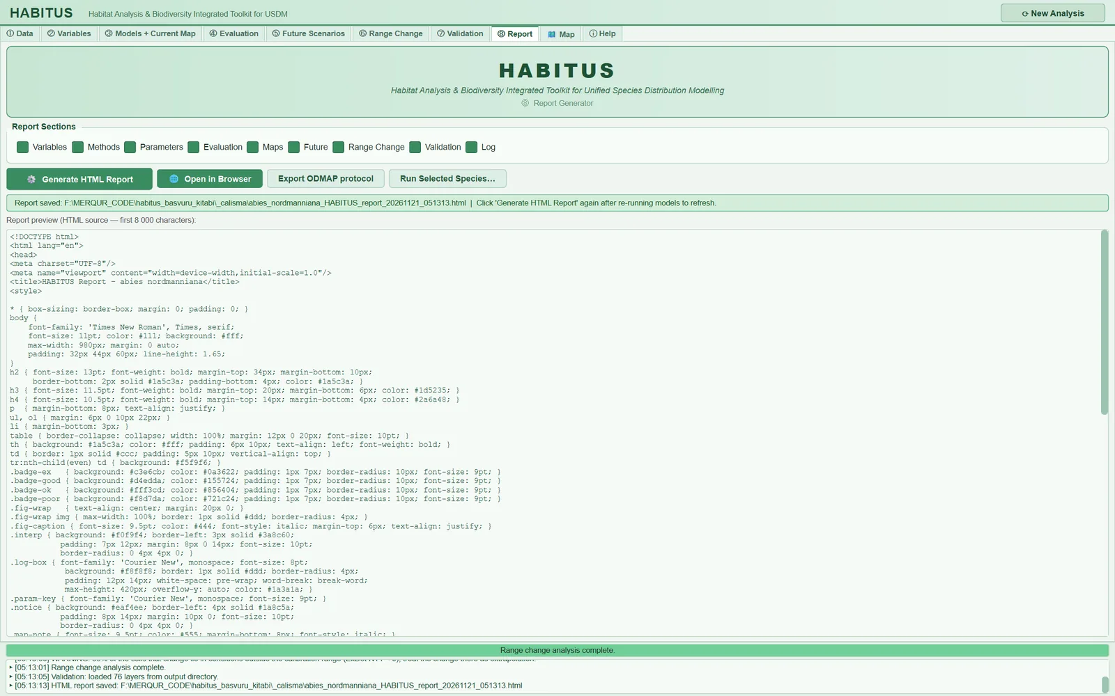
The tab has a single pane (tabs/tab_report.py:376-465). From top to bottom: the header box, Report Sections (section selection, §11.3), four buttons (§11.4, §11.6, §11.8), the progress bar and status line, and the Report preview (HTML source — first 8 000 characters): preview box.

11.3 Report options (Report Sections)
| Name in the UI | What it does | Default | Range / options | Code |
|---|---|---|---|---|
Variables |
Section 2: variable screening and selected variables | on | on / off | tabs/tab_report.py:400, :2416-2418 |
Methods |
Section 3: methods text | on | on / off | :401, :2421-2423 |
Parameters |
Section 4: table of general settings and algorithm settings | on | on / off | :402, :2426-2428 |
Evaluation |
Section 5: evaluation tables and plots | on | on / off | :403, :2431-2433 |
Maps |
Section 6: current map PNGs saved by the user | on | on / off | :404, :2436-2439 |
Future |
Section 7: map PNGs in the scenario folders | on | on / off | :405, :2443-2448 |
Range Change |
Section 8: range-change tables and maps | on | on / off | :406, :2464-2467 |
Validation |
Section 9: ⑦ Validation results | on | on / off | :407, :2470-2473 |
Log |
Section 10: session log | on | on / off | :408, :2476-2481 |
- What it does. Each box adds or removes one section of the report. Section 1 (Study Summary), the environmental novelty section (ExDet) and the processing notices are always added, regardless of the boxes (
tabs/tab_report.py:2412-2413,:2450-2461): these three sections cannot be switched off because they determine how the maps are to be read. - When and how to set it. If a complete report is wanted as supplementary material, all are left on. If only the methods and evaluation are to be taken into the main text, the file can be made smaller by switching off
Maps,FutureandLog(embedded PNGs and a long log increase the size; the example report is 5.5 MB). - Effect on results. It does not change any computation. Even if a box is ticked, the section is not written if its source is missing: for example, if ⑦ Validation was not run, section 9 does not enter the report, and if no map PNG was saved, sections 6 and 7 do not (sections 6, 7 and 9 are absent from the example report).
- Caution. The boxes do not select variables, or which scenario or which range-change analysis enters the report; all scenarios and range-change analyses in the session are written.
11.4 Generate HTML Report and Open in Browser
| Name in the UI | What it does | Default | Range / options | Code |
|---|---|---|---|---|
⚙ Generate HTML Report |
Generates the report from scratch and saves it to the output folder | — | — | tabs/tab_report.py:417-419, :2365-2539 |
🌐 Open in Browser |
Opens the most recently generated report in the system's default browser | disabled until a report is generated | — | :420-421, :2541-2547 |
On every click all outputs are re-read and the report is built from scratch; the status line says so: Each click re-reads all outputs and re-generates from scratch. (tabs/tab_report.py:449-451). The file name is <species>_HABITUS_report_<timestamp>.html; every generation writes a new file and older ones are not deleted (tabs/tab_report.py:2507-2510). If there is no output folder, a save dialog opens. When the job is finished, the Report Ready window shows the path and the first 8000 characters of the HTML source are written to the preview box. In the example run the report was saved as abies_nordmanniana_HABITUS_report_20261121_051313.html.
Tip: If a model or scenario has been re-run, the report is not updated automatically;
Generate HTML Reportmust be clicked again.
11.5 Sections of the HTML report
The report is in English and is written as a draft of supplementary material to be submitted to a journal; the note at the very top says so explicitly: Results and interpretive text should be reviewed and adapted before submission to a scientific journal. (tabs/tab_report.py:2405-2409). The sections and their contents are given below.
11.5.1 Header and 1. Study Summary
The header contains the species name (in italics) and the time of generation. Section 1 is a table: target species, number of records after filtering (number of presences in the first pseudo-absence set), number of variables, algorithms, total number of models, output folder and date of generation (tabs/tab_report.py:703-725). In the example run: 143 records, 8 variables, 4 algorithms.
11.5.2 2. Selected Variables and Multicollinearity Assessment
The screening method in ② Variables (VIF and |r| thresholds, correlation method) is described in a paragraph; if any of the selected variables exceeds the VIF threshold, they are reported by name. 2.1 Variable Screening Table lists, for each candidate variable, the VIF, the univariate AUC, and VIF and correlation eligibility; 2.2 Final Selected Variables lists the selected variables. The correlation heat map in the figures\ folder (that of the selected variables, if it exists) and the VIF bar chart are embedded (tabs/tab_report.py:729-878).
11.5.3 3. Methods
The methods section builds sentences from the settings actually used in the session (tabs/tab_report.py:879-1205):
3.1 Occurrence data: filtering steps and the number of records remaining.3.2 Environmental predictors: the selected variables.3.3 Absence and background data: absence source (pseudo-absence, user absences or both), number and size of sets; accessible area (buffer/hull method and kilometre value, or user polygon and how many of its units were selected; percentage of the extent); thinning distance, its source and the records remaining; same-cell filtering.3.4 Modelling algorithms: algorithm descriptions and references; cross-validation design (spatial block, environmental block, other designs or random) and a caution on how the design affects the scores; mean spatial sorting bias (SSB); number of merged folds.3.5 Ensemble modelling: two-level or single-level combining, number of replicates per algorithm, combining rule.3.6 Model evaluation: AUC, TSS, Boyce, calibration measures and a caution depending on the absence source.3.7 Reproducibility: random seed and a reference to thehabitus_run_config.jsonfile.
11.5.4 4. Model Parameters
The Global Modelling Settings table (selected variables, pseudo-absences per set, pseudo-absence strategy, number of sets, number of folds, training/test ratio, permutation-importance repeats) and the 4.1 Algorithm Settings table (full name, reference, description and hyperparameters of each algorithm) (tabs/tab_report.py:1209-1267).
Caution: The
Pseudo-absences per replicateandPA strategyrows in this table do not show the values chosen in ① Data but the defaults 1000 andrandom; the correct values are found in the text of section 3.3 and in thehabitus_run_config.jsonfile (settings.background). TheTrain / Test splitrow is not used in the spatial block design; the fold arrangement is described in 3.4.
11.5.5 5. Model Evaluation Results
First, the cautions that determine how the scores are to be read (random folding, spatial sorting bias, etc.) are given before the table (tabs/tab_report.py:1271-1392). Then: 5.0 Performance and its variability (spread across replicates), 5.1 Individual Model Scores (AUC, TSS, Boyce, threshold, prevalence, calibration slope and interpretation for each model and fold), 5.1a Ensemble Scores (scores of the ensemble on the cross-validation held-out folds), 5.1b Threshold-based Metrics and Omission Rates (Kappa, MCC, sensitivity, specificity, Jaccard, Sørensen, FPB, omission rates, ΔAUC), 5.2 Algorithm Summary (algorithm mean ± SD) and, under the 5.3 subheadings, the evaluation, ROC, omission/precision-recall/calibration, variable importance and response curve plots from the figures\ folder. These outputs are detailed in Chapter 7.
11.5.6 6. Current Distribution
The report does not draw the current map GeoTIFFs; it embeds the PNG files the user has saved from the map viewer. All PNGs in the root of the output folder are taken, except those whose names start with habitus_ and end with _study_area.png (tabs/tab_report.py:1794-1880). The map type is guessed from the file name (prob/suitability → suitability, bin → binary, range/src → range change) and a ready-made interpretive paragraph is added accordingly.
Caution: The save dialog of the viewers in ⑤ and ⑥ also opens by default in the root of the output folder (
map_widget.py:612-620). A future map saved there appears in this section under the heading "Current Distribution". Save future maps in the scenario subfolder (§11.5.7).
11.5.7 7. Future Scenarios
Every subfolder in the output folder (except figures, validation and current) is treated as a period; for every subfolder that contains PNGs, a 7.k <folder name> heading is opened and the PNGs are embedded (tabs/tab_report.py:1884-1973). The folder name is the scenario name (the Output subdir in ⑤, or the scenario name if that is empty). If there are no PNGs at all, the section is not written.
11.5.8 7.1 Environmental Novelty (Extrapolation Detection)
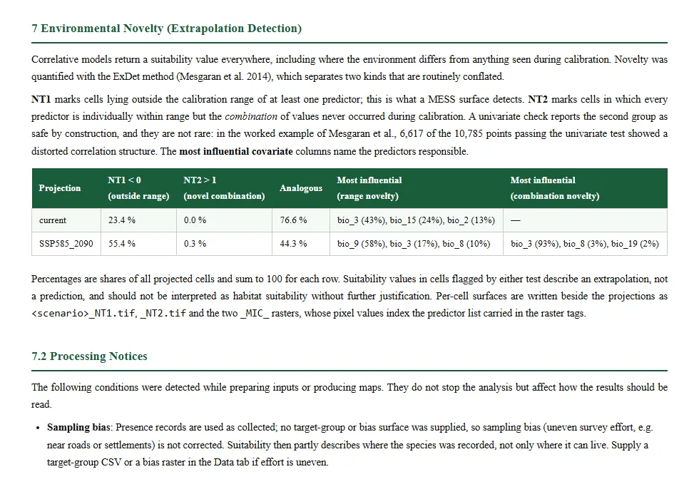
For each projection (current first, then the scenarios alphabetically), NT1 < 0, NT2 > 1, the percentage of cells that are similar under both tests and the three most influential variables for range/combinatorial novelty are tabulated; if NT2 could not be computed, the reason is given (tabs/tab_report.py:2024-2123). If the future section (7) was not written, the heading becomes 7 Environmental Novelty …. The method is described in Section 8.9.
11.5.9 7.2 Processing Notices
Situations that change how the maps are read but do not stop the job are itemized here; if there are none, the section is not written (tabs/tab_report.py:1981-2022):
- layers aligned to the training grid in projections, and warnings about uncovered cells (§8.10);
- a future map aligned in range change;
- the sampling-bias warning (if no target group or bias surface was given; this is the only note in the example report);
- the selection-bias note, if a tuning search was run;
- the reason, if the ensemble map could not be produced;
- data input and validation notes.
11.5.10 8. Range Change Analysis
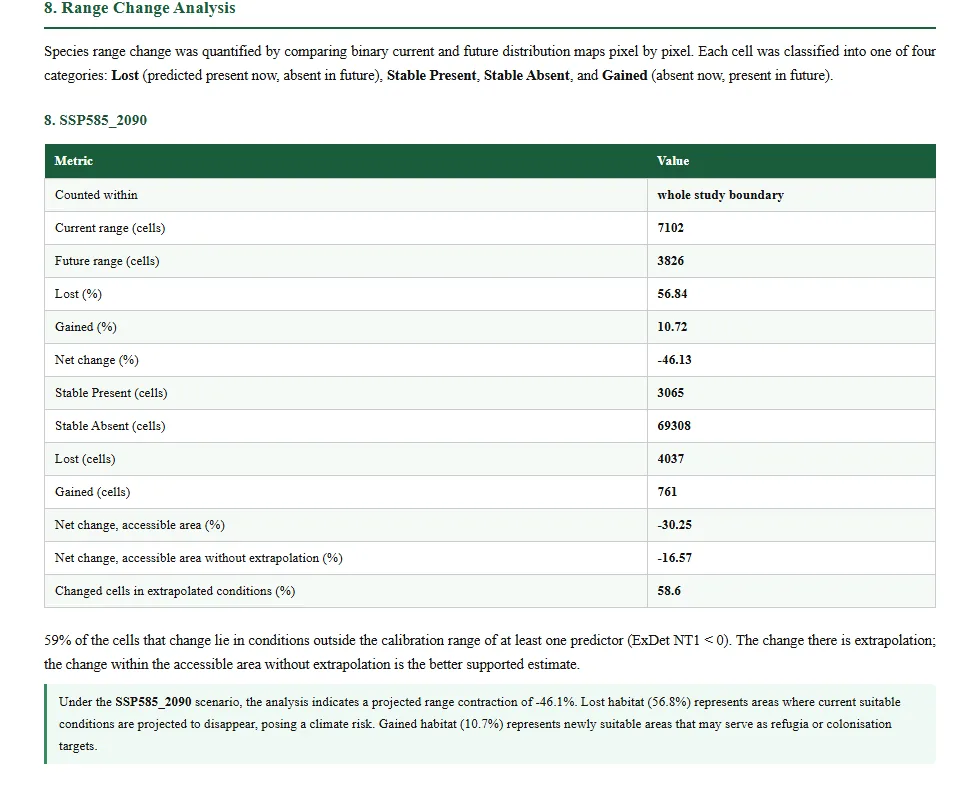
For each range-change analysis: a subheading, the same rows as the table in ⑥ (extent, current and future area, percentages, cell counts, net change of the other extents, share of change under extrapolation), a note if 25% or more of the changed cells lie in extrapolated conditions, a three-level interpretation based on net change (below −10 contraction, above +10 expansion, in between stability) and a colour map redrawn from the _SRC.tif file (tabs/tab_report.py:2126-2265).
11.5.11 9. Validation
If a validation was carried out in ⑦ Validation: mode, reference and validation layers, number of points, overall accuracy, Cohen's κ, weighted F1 (R², RMSE, MAE if available), confusion matrix and at most two maps from the validation\reclassify*.tif files (tabs/tab_report.py:2269-2359). Details are in Chapter 10.
11.5.12 10. Session Log and citation
Of the .log files in the output folder, the one with the greatest name (the newest session) is written as is into a scrollable box (tabs/tab_report.py:606-614, :2476-2481). The recommended citation for HABITUS is at the end of the report (tabs/tab_report.py:2484-2495).
Note: The log is written to a new file in every session. If the program was closed and reopened with the same output folder, only the log of the last session enters the report; the records of the previous session remain in their own
.logfile.
11.6 ODMAP export (Export ODMAP protocol)
| Name in the UI | What it does | Default | Range / options | Code |
|---|---|---|---|---|
Export ODMAP protocol |
Writes the odmap_protocol.md and odmap_protocol.csv files to the output folder |
— | — | tabs/tab_report.py:422-430, :537-570 |
- What it does. ODMAP (Overview, Data, Model, Assessment, Prediction) is the standard protocol proposed for reporting species distribution models (Zurell et al. 2020). The button builds the 79 elements of the protocol's Table 1 row by row; it fills in the elements for which a record exists in the
habitus_run_config.jsonfile and the session (auto), and marks the rest asuser_required(odmap.py:42-111,:156,:637-686). No value is invented; the tooltip text also states that the report will not count as ODMAP-compliant until the user has filled in these rows. - When and how to set it. Before submitting a paper; the file is written only when the button is clicked, not automatically (
tabs/tab_report.py:538-540). The models and projections should be completed first, then exported. - Effect on results. It does not affect the computation. In the example run 46 of the 79 elements were filled in automatically and 33 were left to the user. The status line and the log write the following message:
ODMAP protocol written (79 elements: 46 filled automatically, 33 to be completed by you): …. - Caution. If there is no output folder, the message
No output folder yet. Run the models first.appears. Ifhabitus_run_config.jsoncannot be found, all elements becomeuser_requiredand a note to that effect is added to the message (tabs/tab_report.py:552-564).
Main elements filled in automatically (from the example run): model objective (algorithms, binary map rule), species name, location and grid (rows × columns, cell size, coordinate system), type of extent boundary (accessible-area buffer), response type (presence-pseudo-absence), variables, algorithms and ensemble method, summary of the steps, software and package versions, sample size and filtering rationale, pseudo-absence settings and seed, training/validation partitioning (including block size), variable pre-selection, algorithm settings, setting for prediction beyond the sampled range (clamping), variable importance, ensemble weights, how spatial autocorrelation was addressed, threshold rule, performance statistics, prediction unit, uncertainty maps, transfer scenarios and novelty quantification (ExDet; MESS and its mask if selected).
Elements left to the user: authors, contact, title, DOI; study objective; temporal extent and resolution; observation type; hypotheses and assumptions; rationale for model complexity; code and data availability; taxonomic reference system, ecological level, data sources, sampling design; independent test data; sources, temporal and spatial resolutions and measurement errors of the variables and transfer layers; model coefficients; temporal autocorrelation and nested data; response curves and the outcome of expert judgement; input data and parameter uncertainty. The multicollinearity element is filled in automatically when the thresholds in ② Variables can be read from the session (odmap.py:487-495).
11.7 Publication maps
HABITUS maps are not saved as screenshots of the on-screen viewer but are redrawn at journal column width (map_widget.py:597-668). This saving is done with the floppy-disk icon in the toolbar of the map viewers in ③, ⑤ and ⑥; the study-area map is saved with the 💾 Save study-area figure… button in the 🗺 Map tab (tabs/tab_map.py:124-130, study_area_figure.py:293-313). Both open the same Figure for publication dialog (map_widget.py:180-238).
| Name in the UI | What it does | Default | Range / options | Code |
|---|---|---|---|---|
Width: |
Printed width of the figure | Double column — 174 mm |
Single column — 85 mm, 1.5 column — 120 mm, Double column — 174 mm |
map_widget.py:112-116, :306 |
Resolution: |
Resolution in raster formats | 600 dpi |
300 dpi, 600 dpi, 1200 dpi |
map_widget.py:117, :197-203 |
Title: |
Title text (study-area map only) | species name | free text | map_widget.py:209-212 |
Include the title above the map |
Writes the title above the map | on (result maps), off (study area) | on / off | map_widget.py:204-206, :306, tabs/tab_map.py:139 |
Italic title (scientific name) |
Writes the title in italics (study area) | on if a species name exists | on / off | tabs/tab_map.py:289 |
Locator map in the upper-left corner |
Locator inset map (study area) | on | on / off | tabs/tab_map.py:290 |
| file type | Format in the save dialog | PNG | PNG, TIFF (LZW), PDF, SVG, EPS, JPEG | map_widget.py:156-177 |
The print layout is drawn with Arial 7–9 pt, a white background and thin lines; fonts are embedded in PDF/SVG/EPS (map_widget.py:126-131, :149-153). Resolution is not used in vector formats (PDF, SVG, EPS). The height of the map is computed from the geographic aspect ratio (with latitude cosine correction) and limited to at most 9 inches (map_widget.py:652-662). The study-area map draws the records, the boundary, a scale bar and a north arrow over the Natural Earth country boundaries embedded in the package (study_area_figure.py:1-10). The viewer's other controls are described in Chapter 12.
Tip: Sections 6 and 7 of the report embed only PNG files. If PDF/TIFF is to be saved for a journal, save the same map once more as PNG (the current map to the root of the output folder, the future map to the scenario subfolder). The report text states "300 DPI" for these maps; the default of the save dialog is 600 dpi.
11.8 Multi-species batch run (Run Selected Species…)
| Name in the UI | What it does | Default | Range / options | Code |
|---|---|---|---|---|
Run Selected Species… |
Repeats the completed workflow with the same settings for the other species ticked in ① Data | — | confirmation dialog | tabs/tab_report.py:431-438, :469-512, batch_species.py |
- What it does. In an occurrence file containing several species, after the workflow has been completed manually for one species, the other species ticked in ① Data are processed in turn. The steps repeated for each species (
batch_species.py:145-159): 1. ① Data: the active species is changed and data preparation is run with the same settings; 2. ② Variables: the variables selected for the first species (and the categorical selection) are assigned unchanged; a warning on the number of variables relative to this species' number of records is written to the log (batch_species.py:201-224); 3. ③ Models: models are fitted using the tab's settings as they are (including the current map); 4. ⑤ each scenario: with the same raster list, algorithms, subfolder, MESS, mask and clamping choice (batch_species.py:226-239); 5. ⑥ each range-change analysis: the keys selected from the list (e.g.current :: EMwmean_bin) are translated to this species' files, with the same analysis name and extent (batch_species.py:241-259); 6. ⑧ HTML report.
The output folder per species has the form <output folder>\<species> (tabs/tab_data.py:1115-1124).
- When and how to set it. First the workflow is carried out completely and carefully for one species; every analysis to be reported in ⑤ and ⑥ must have been run once, because the batch run repeats only what has been run in the session. The confirmation dialog lists the species to be repeated, the variables, and the number of scenarios and range-change analyses (tabs/tab_report.py:489-499).
- Effect on results. Each species gets the result it would have got if it had been done manually; the program does not use a separate pipeline but drives the tabs themselves (batch_species.py:12-15). Variable selection, however, is not redone per species: the first species' selection is applied to all species.
- Caution. All message windows that open during the run are answered automatically (Yes to question dialogs) and written to the log with the prefix [batch, …] (batch_species.py:80-111). If a step fails, the remaining steps for that species are skipped and the run moves on to the next species. When the job is finished, <output folder>\batch_summary.csv is written: species, status (done / failed), failed_step, error (the user-facing last line of the error), output_dir, minutes (batch_species.py:263-302). If this file is open in another program it cannot be written, and a note is added to the log.
Not repeated in a batch run: the tuning search step, ⑦ Validation, ODMAP export and the saving of map PNGs. For this reason sections 6, 7 and 9 are absent from the reports of the species in a batch run. In addition, there is no button in the UI to interrupt a batch run; the job continues until all species are finished.
Messages: if no species is ticked, The batch run is for an occurrence file with several species: tick the species to analyse in ① Data.; if the workflow has not been completed, Complete the workflow for one species first (at least ① Data, ② Variables and ③ Models); …; if the only ticked species is the one already processed, No other species is ticked in ① Data. (tabs/tab_report.py:474-487).
11.9 Outputs
<species>_HABITUS_report_<time>.html: single-file report with embedded images.odmap_protocol.md,odmap_protocol.csv: partly filled ODMAP (CSV columnssection, subsection, element, value, source).- In a batch run:
<species>\subfolders andbatch_summary.csv. - Saved publication maps: at the path chosen by the user.
11.10 Expert questions
Q1. Can the methods text in the report be put directly into a paper?
Answer: The report itself does not recommend this: the note at its beginning says that the text should be reviewed and adapted (tabs/tab_report.py:2405-2409). The text is built from the actual settings in the session (e.g. accessible area, thinning, fold design and SSB, tabs/tab_report.py:930-1092), but the statements of principle and the citations are generic templates; the pseudo-absence rows in section 4 also show default values (§11.5.4). The numbers should be checked against habitus_run_config.json.
Q2. Does the ODMAP output count as "ODMAP-compliant"?
Answer: No. The module uses only the elements in Table 1 of Zurell et al. (2020); the full question list in Supplementary Table A1 was not used, and the file states this explicitly (odmap.py:11-21, :661-664). In the example run 33 elements must be filled in by the user. Completing it by comparison with the form in the ODMAP Shiny app is recommended.
Q3. Is the MESS or clamping choice visible in the report?
Answer: Not in the HTML report; the novelty section tabulates only the ExDet results (tabs/tab_report.py:2024-2123). The choices are found in ODMAP ("Settings for extrapolation beyond sample range", "Quantification of novel environments", odmap.py:466-508) and in the _projection_options.json file in each scenario folder. These choices need to be stated in the methods part of the paper.
Q4. What is the denominator of the ExDet percentages in the report?
Answer: All cells predicted in the projection (with all variables finite); the NT1 < 0, NT2 > 1 and similar percentages sum to 100 (sdm_novelty.py:100-125, report note tabs/tab_report.py:2109-2118). The NT2 percentage is also divided by all cells, not by the subset in which NT2 was computed. In the example run, for SSP585_2090: 55.4 + 0.3 + 44.3 = 100.
Q5. In a batch run, is variable selection redone for each species?
Answer: No; the variables confirmed in ② Variables for the first species are assigned unchanged (batch_species.py:201-218). The program only writes to the log whether this species' number of records is sufficient for that many variables (note_selected_predictors, batch_species.py:219-224). If the species differ in ecology or their numbers of records differ greatly, variable selection should be done manually per species and the species run separately. In biomod2, batch work is done with a loop written by the user; the HABITUS counterpart is applying the same settings to all species.
Q6. In a batch run, if one species fails, are the others affected?
Answer: No. The failed step is recorded, the remaining steps for that species are skipped and the run moves on to the next species (batch_species.py:161-190, :263-274). batch_summary.csv records at which step and why it failed; the user-facing last line of the error text is taken (batch_species.py:26-51). The full traceback remains in the log with the prefix [batch, trace].
Q7. Which resolution should be chosen for publication maps?
Answer: The dialog tooltip recommends 300 dpi for colour maps in general and 600 dpi or more for figures with fine text and lines (map_widget.py:201-203); the default is 600 dpi. In vector formats (PDF, SVG, EPS) dpi is not used; the raster layer is still embedded as an image. The column widths are the common sizes of Elsevier, Wiley and Springer (85, 120, 174 mm; map_widget.py:111-116); if the journal's own size is different, the nearest width should be chosen and scaled according to the journal guidelines.
Q8. Where do the map interpretation paragraphs in the report come from?
Answer: They are fixed texts chosen according to the file name (tabs/tab_report.py:1824-1865, :1935-1958): for example, for a probability map, a suggestion to prioritize areas of high suitability for fieldwork; for a future map, a sentence about a northward/upward shift with warming. These sentences are not derived from the data themselves; they should be rewritten according to the findings before being taken into a paper. The range-change interpretation, by contrast, is built from the actual value of the net change (±10% thresholds) (tabs/tab_report.py:2184-2196).
Q9. Is the report reproducible; which files are sufficient?
Answer: The report is generated from scratch from the session results on every click; after the session is closed the same report cannot be regenerated, because the models and the ExDet summaries are held in memory. For reproducibility, habitus_run_config.json (all settings, seed, package versions), the _projection_options.json files in the scenario folders and the saved HTML report should be kept together. Section 3.7 states the seed and the configuration file (tabs/tab_report.py:1138-1151).
Q10. How many scenarios and how many range-change analyses appear in the report?
Answer: All those carried out in the session. The novelty table writes every projection in state["novelty"], and section 8 every analysis in state["range_results"] (tabs/tab_report.py:2044-2073, :2140-2207). If there is a trial that should not enter the report, the results should be reset with Remove All in ⑤ and only the desired ones re-run.
11.11 Common mistakes and pitfalls
- Not saving the maps as PNG. The report does not draw current or future maps from the GeoTIFFs; if no PNG was saved, sections 6 and 7 do not appear at all.
- Saving a future map to the root of the output folder. It appears in the report under "6. Current Distribution".
- Trusting the pseudo-absence rows in section 4. The correct values are in section 3.3 and in the
habitus_run_config.jsonfile. - Assuming the ODMAP file is complete. Until the
user_requiredrows are filled in, the file is not an ODMAP report. - Starting a batch run with a workflow that has not been completed for one species. Only the scenarios and range-change analyses run in the session are repeated; if no scenario was run in ⑤, no future map is produced in the batch run either.
- Overlooking the variable warning in a batch run. For species with few records,
[batch] ADVISORY:lines appear in the log; the number of variables may be too high for that species. - Forgetting to regenerate the report. A new scenario or refitted models enter the report only when
Generate HTML Reportis clicked again; the old file is not deleted, and a new time-stamped file is written.
11.12 References
Zurell, D., Franklin, J., König, C., Bouchet, P.J., Dormann, C.F., Elith, J., Fandos, G., Feng, X., Guillera-Arroita, G., Guisan, A., Lahoz-Monfort, J.J., Leitão, P.J., Park, D.S., Peterson, A.T., Rapacciuolo, G., Schmatz, D.R., Schröder, B., Serra-Diaz, J.M., Thuiller, W., Yates, K.L., Zimmermann, N.E., Merow, C., 2020. A standard protocol for reporting species distribution models. Ecography 43, 1261–1277. https://doi.org/10.1111/ecog.04960