6. Models II: cross-validation, threshold, ensemble and results (③ Models)
Tab: ③ Models + Current Map · Code: tabs/tab_models.py, tabs/tab_tuning.py (UI); sdm_core.py SDMModeler, EnsembleModeler, Projector, evaluate_all; sdm_spatial.py (blocks, variogram, folds, SSB); sdm_tuning.py (grid search)
6.1 What this tab does
The ③ Models tab fits the selected algorithms with the predictors chosen in the ② Variables step, tests each of them by cross-validation (CV), projects the models refitted on all data onto the current climate layers, and combines them into an ensemble map. Chapter 5 describes the algorithms' own options (Algorithm Options); this chapter describes everything else on the same tab: which algorithms run, how the data are split into folds, how the binary (presence/absence) threshold is chosen, how the ensemble is built, the optional tuning search, and the result sub-tabs.
- Input: the pseudo-absence (PA) sets produced in ① Data, the continuous and categorical predictors confirmed in ② Variables, the training rasters and the seed. If these are missing, the button gives the message
"Complete ① Data and ② Variables steps first."(tabs/tab_models.py:1394-1395). - Output: evaluation scores for each algorithm × PA set × CV run; probability and binary maps of the models fitted on all data (
Full); mean and spread maps per algorithm;EM*ensemble maps;evaluation_scores.csv,habitus_run_config.json, training/test point files (§6.10). - Lock order: when the run finishes, the ④ Evaluation, ⑤ Future Scenarios, ⑥ Range Change, ⑦ Validation and ⑧ Report tabs are unlocked (
tabs/tab_models.py:1848-1852).
A single button, ▶ Run Models + Generate Current Distribution Map, does four jobs in sequence (tabs/tab_models.py:1559-1659): (1) CV and full-data models with SDMModeler.run(), (2) filtering of ensemble members with EnsembleModeler, (3) projection onto the current climate and writing of the maps with Projector.project(), (4) writing of the run record (habitus_run_config.json).
6.2 Screen layout
Figure 6.1. The ③ Models + Current Map tab before a run: four sub-tabs at the top, Select Algorithms on the left, Algorithm Options on the right, the Training Settings and Combining Results && Binary Threshold Method boxes below, and the run button at the very bottom.
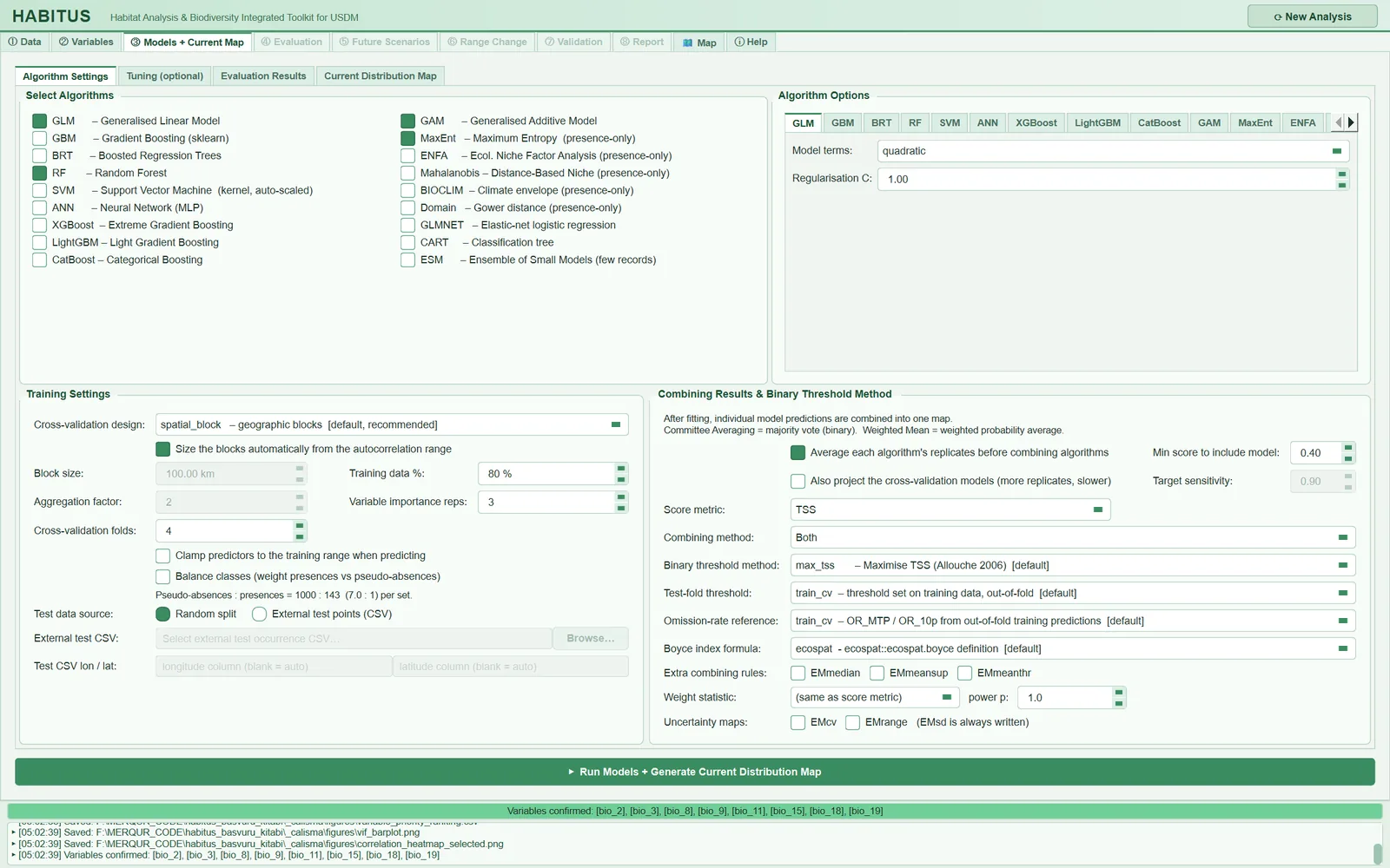
The tab has four sub-tabs and a single run button that stays below all of them (tabs/tab_models.py:91-110):
| Region | Content | In this chapter |
|---|---|---|
Algorithm Settings |
Select Algorithms, Algorithm Options, Training Settings, Combining Results && Binary Threshold Method |
§6.3–6.6 (algorithm options: Chapter 5) |
Tuning (optional) |
Grid search for a single algorithm | §6.7 |
Evaluation Results |
ROC-AUC, TSS, Boyce table per model | §6.8 |
Current Distribution Map |
Status text, table of produced maps, output folder, map viewer | §6.9 |
| Bottom strip | ▶ Run Models + Generate Current Distribution Map |
§6.1 |
When the run starts, the program switches to the Evaluation Results sub-tab, and when it finishes it opens the Current Distribution Map sub-tab (tabs/tab_models.py:1491, 1835).
6.3 Algorithm selection (Select Algorithms)
Figure 6.2. The Select Algorithms box: eighteen algorithms in two columns; GLM, RF, GAM and MaxEnt are ticked in the example run.
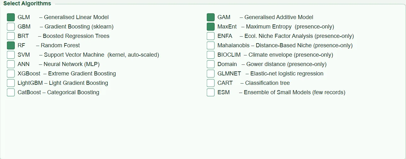
The box contains eighteen check boxes; each adds one algorithm to the run list (tabs/tab_models.py:125-150). Every box that is ticked and enabled runs (tabs/tab_models.py:1397-1398). If none is selected, the message "Select at least one algorithm." appears.
| Name in the UI (short) | What it does | Default | Code |
|---|---|---|---|
GLM, RF |
Generalized linear model; random forest | on | tabs/tab_models.py:129-132 |
GBM, BRT, SVM, ANN |
Gradient boosting (sklearn), boosted regression trees, support vector machine, multilayer neural network | off | tabs/tab_models.py:130-134 |
XGBoost, LightGBM, CatBoost |
Three boosting libraries; if not installed the box is greyed out and shows [not installed] |
off | tabs/tab_models.py:135-137, 152-168 |
GAM |
Generalized additive model (requires pygam) | off | tabs/tab_models.py:138 |
MaxEnt, ENFA, Mahalanobis, BIOCLIM, Domain |
Presence-only methods | off | tabs/tab_models.py:139-143 |
GLMNET, CART, ESM |
Elastic-net logistic regression, classification tree, ensemble of small models | off | tabs/tab_models.py:144-146 |
What it does. Each selected algorithm is fitted on every PA set, in every CV fold, and once more on all data (sdm_core.py:5409-5643, 5654-5768). The ensemble map consists only of the selected algorithms (sdm_core.py:7844-7855).
When and how to set it. The ensemble approach envisages combining algorithms with different biases (Araújo and New 2007); adding algorithms that are very similar to one another (e.g. GBM, BRT, XGBoost and LightGBM all together) weights the ensemble towards a single family. Two-level combining (§6.6.1) removes this effect with respect to the number of replicates, but not with respect to the number of families. For species with few records (roughly fewer than 30 presences), ESM and the presence-only methods are meaningful (Chapter 5).
Effect on results. Run time grows linearly with the number of algorithms: the total number of fits is roughly algorithms × PA sets × (folds + 1); when Test-fold threshold = train_cv, three inner fits are added to every CV fit (§6.5.2). In the example run the MaxEnt full model alone took 25–28 s (session log).
Caution. The default the program loads itself is GLM and RF only; the four algorithms in the figure were ticked by hand for the example run.
6.4 Training settings (Training Settings)
Figure 6.3. The Training Settings box with default values: spatial_block design, automatic block size (Block size and Aggregation factor greyed out), 4 folds, Random split, and the Clamp/Balance boxes off.
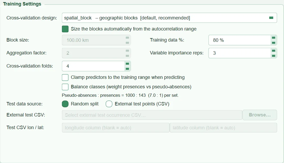
This box determines how the data are split into training and test parts. HABITUS produces its scores from the held-out part of the cross-validation folds; the choice of design therefore directly affects all reported scores.
| Name in the UI | What it does | Default | Range / options | Code |
|---|---|---|---|---|
Cross-validation design: |
Fold design | spatial_block |
8 designs (§6.4.1) | tabs/tab_models.py:219-255 |
Size the blocks automatically from the autocorrelation range |
Takes the block size from the variogram range | on | on / off | tabs/tab_models.py:265-271 |
Block size: |
Manual block side length | 100 km (only when automatic is off) | 1–5000 km | tabs/tab_models.py:273-279 |
Aggregation factor: |
Checkerboard cell multiplier | 2 | 1–20 (only checkerboard*) |
tabs/tab_models.py:256-263 |
Cross-validation folds: |
Number of folds | 4 | 1–10 (greyed out for jackknife) |
tabs/tab_models.py:211-216 |
Clamp predictors to the training range when predicting |
Clamps predictors to the training range | off | on / off | tabs/tab_models.py:354-364 |
Balance classes (weight presences vs pseudo-absences) |
Weights the classes inversely to their size | off | on / off | tabs/tab_models.py:333-352 |
Test data source: |
Source of the test data | Random split |
Random split / External test points (CSV) |
tabs/tab_models.py:294-299 |
Training data %: |
Training share in the fallback evaluation split | 80 % | 50–95 % | tabs/tab_models.py:301-303 |
External test CSV: |
External test file | empty | CSV file | tabs/tab_models.py:305-311 |
Test CSV lon / lat: |
Coordinate columns in the external test file | empty (automatic) | column name | tabs/tab_models.py:313-320 |
Variable importance reps: |
Number of permutation-importance repeats | 3 | 0–10 | tabs/tab_models.py:290-291 |
The enabling rules are in the _toggle_block function (tabs/tab_models.py:281-289): the block boxes are enabled only for spatial_block, checkerboard and checkerboard2; Aggregation factor only in the checkerboard designs; Cross-validation folds in every design except jackknife.
6.4.1 Cross-validation design (Cross-validation design)
What it does. For each PA set it assigns a fold number to every row (SDMModeler._build_folds, sdm_core.py:4997-5162). Fold k becomes the test set in turn and the remaining folds form the training set (sdm_core.py:5429-5450). There are eight designs:
| Option | How the folds are formed | Code |
|---|---|---|
spatial_block |
A square grid is laid over the study area; each block is assigned as a whole to one fold. Blocks are distributed by the best of 50 seeded trials so that the numbers of presences and absences in each fold are balanced | sdm_spatial.py:385-511, 305-357 |
environmental |
Predictors are standardized and split into folds clusters with k-means; each cluster is one fold |
sdm_spatial.py:514-558 |
random |
Random folds stratified by class | sdm_spatial.py:561-580 |
checkerboard |
Checkerboard with cell side = block size × Aggregation factor; two colours, two folds |
sdm_spatial.py:623-706 |
checkerboard2 |
Two checkerboards, fine (block size) and coarse (block size × factor); fold = 2 × coarse colour + fine colour, four folds | sdm_spatial.py:666-672 |
jackknife |
Each presence is its own fold; absences are distributed equally and randomly among the folds | sdm_spatial.py:709-755 |
lon_bands / lat_bands |
folds bands along longitude or latitude with equal numbers of presences |
sdm_spatial.py:758-790 |
In addition, if Test data source: = External test points (CSV) is selected, the folds are not used for testing (§6.4.5).
When and how to set it. With clustered records, a random split leaves a training point right next to a test point carrying almost the same predictor values, and inflates the scores (Roberts et al. 2017). This is why the default is spatial_block. If projections to future climate are planned, environmental tests transfer to conditions the model has not seen more directly. checkerboard and checkerboard2 correspond to the partitions of the same name in ENMeval (Muscarella et al. 2014): test and training points are interleaved throughout the area. jackknife is for species with fewer than about 25 presences (sdm_spatial.py:594; Pearson et al. 2007). Bands test transfer along a latitudinal or longitudinal gradient. random should be kept only for reproducing an earlier result or for comparison.
Effect on results. The design determines every reported score (AUC, TSS, Boyce), the members entering the ensemble (§6.6.4) and the members' weights, because the score of the Full models is the mean of the CV folds (sdm_core.py:5818-5853). Blocked designs give lower but more honest scores than a random split.
Caution.
- If the design cannot be applied (too few blocks, folds that do not contain both classes, no coordinates), the program falls back to random folds and writes this to the log and the report with the note
"WARNING (design not applied): …"; the summary line shows[BLOCKING FAILED - scores are optimistic](sdm_core.py:5135-5140,5933-5934). - Folds containing no presences or no absences are merged into another fold; in this case fewer folds than requested are evaluated and the message
"WARNING: … requested folds held no presence or no absence and were merged into others …"is given (sdm_core.py:5124-5134;sdm_spatial.py:360-382). - In the
randomdesign the number of folds cannot exceed the number of records of the rarer class (sdm_spatial.py:572-574). - In the checkerboard designs the number of folds is fixed (2 or 4); in these designs
Cross-validation folds:only limits how many folds are run (sdm_core.py:5400-5401). Withcheckerboard2, a value below 4 leaves some folds never tested; keep the number of folds at 4 in this design.
6.4.2 Block size: automatic or manual
What it does. When Size the blocks automatically from the autocorrelation range is on, the block side is the empirical variogram range computed in the ① Data stage from the predictor values at the presence points (sdm_core.py:2433-2462, 5096-5106). The computation is as follows (sdm_spatial.py:166-281): at most 1500 points are subsampled; the semivariance \gamma(h)=\tfrac12\,\overline{(z_i-z_j)^2} is computed in 15 distance classes up to half the largest pairwise distance; the median of the outer third of the classes is taken as the sill; the distance at which \gamma first reaches 95% of the sill is the range of that predictor; the block size is the median of these ranges across predictors. If there are fewer than 20 points or the variogram cannot be built, 1/10 of the largest pairwise distance of the study area is used (method = "fallback_extent"). When the box is off, the Block size: value is used.
When and how to set it. The automatic value is a simplified counterpart of the logic in blockCV (Valavi et al. 2019). It is entered manually if the range is to be fixed to a scale stated in a paper (e.g. the width of a mountain range) or for comparison with another study.
Effect on results. As the block grows, leakage between folds decreases, scores fall and the difference between folds grows. In the example run the variogram range is 151.5 km and the study-area width 606 km; four folds were built from 30 blocks, with 43/33/35/32 presences in the folds (habitus_run_config.json).
Caution. If the area does not hold as many blocks as the requested number of folds, the block can be halved up to six times; in this case the note reads "Block reduced from … km so that the study area could hold … folds …" (sdm_spatial.py:454-464, 503-507). This reduction applies to both the automatic and the manually entered size. The grid is built in degrees, with the longitude spacing corrected by \cos\varphi at the mean latitude (sdm_spatial.py:439-446).
6.4.3 Aggregation factor (Aggregation factor)
What it does. For checkerboard, cell side = block size × factor; for checkerboard2, fine grid = block size, coarse grid = block size × factor (at least 2) (sdm_spatial.py:651-672). If the block size is automatic, it is the variogram range.
When and how to set it. It plays the same role as aggregation.factor in ENMeval (Muscarella et al. 2014). The default of 2 is sufficient in most cases; increasing it enlarges the checkerboard cells and moves test points away from training points.
Effect on results. A large factor gives a more pessimistic (more independent) test; with a very large factor some colours may contain only one class and the cell is reduced.
Caution. If each fold does not contain both classes, the cell is halved up to six times; if this still fails, the program falls back to random folds (sdm_spatial.py:685-698).
6.4.4 Number of folds (Cross-validation folds)
What it does. It is the number of folds to be formed in the spatial_block, environmental, random and band designs; in all designs it is the upper limit on the number of CV runs (RUN1…RUNk) to be executed (sdm_core.py:5400-5407).
When and how to set it. 4–5 folds are common. As the number of folds increases, each test set shrinks and the variability of the fold scores increases; 3–4 folds are reasonable for small samples, 5 folds for large areas with many records.
Effect on results. Run time grows linearly with the number of folds. The mean and standard deviation of the scores are affected by the number of folds.
Caution. If 1 is selected, the folds are still built as two parts, but only one is tested (sdm_core.py:5018, 5400-5401); in this case the spread of the fold scores cannot be computed and the hold-out score of the ensemble rests on the members' own fold scores (§6.6.9). In jackknife the number of runs equals the number of presences and this field is ignored (sdm_core.py:5402-5406).
6.4.5 Test data source and external test CSV
What it does. When Random split is selected (default), the tests are carried out on the held-out part of the CV folds. When External test points (CSV) is selected, every RUN is trained on all the PA data and tested on the points in the file (sdm_core.py:5417-5427). The coordinate columns are taken from the Test CSV lon / lat: fields; if these are empty, the names longitude/long/lon/lng/decimallongitude/x and latitude/lat/decimallatitude/y are searched for, and if they are not found the 2nd and 3rd columns are used (sdm_core.py:5165-5189). If the file has a column named presence, occurrence or pa, rows with value 0 are treated as true absences; otherwise the test absences are background points newly drawn from the study area, independent of the training; if this also fails, a seeded subsample of the training pseudo-absences is taken and its non-independence is noted (sdm_core.py:5191-5340).
When and how to set it. It is used when records from an independent field survey, another period or another region are available.
Effect on results. The scores rest on independent data; however, because all runs are trained on the same data and tested on the same points, the difference between runs shows only the algorithm's own randomness. The program writes this to the report with the note "External test set: RUN1..RUNn all re-fit the same model on the SAME training data …" (sdm_core.py:5341-5347).
Caution. Test records falling outside the raster or on NoData are counted and reported; if fewer than 10 usable presences remain, the warning "… the test statistics will be very unstable." appears (sdm_core.py:5289-5301). In this mode Training data %: is greyed out and 80 is used (tabs/tab_models.py:1296-1301, 1578). If the run is started without selecting a file, the error "External test points mode selected but no CSV provided." is given.
6.4.6 Training share (Training data %)
What it does. For every model fitted on all data (Full), a random evaluation split is also made: a model is fitted with this percentage of the data and scored on the rest (sdm_core.py:5675-5722). If at least one valid CV score exists for the same algorithm and PA set, this split score is replaced by the mean of the CV folds and Score_source becomes cv_mean (sdm_core.py:5818-5853). The split score is kept only if no CV score was produced at all (Score_source = random_split).
When and how to set it. In normal use there is no need to change it.
Effect on results. When CV succeeds, it has no effect on the reported scores, thresholds or maps.
Caution. The field's tooltip text ("% of occurrence data used for training; remainder used as test set") gives the impression that this setting determines the CV scores; it does not.
6.4.7 Variable importance repeats (Variable importance reps)
What it does. In each CV run, each predictor is permuted in the test fold and the drop in AUC is taken as its importance. For scikit-learn models permutation_importance (n_repeats=3, scoring="roc_auc", fixed seed) is called; in MaxEnt, GAM, ENFA, Mahalanobis, BIOCLIM, Domain and ESM, each predictor is permuted with its own seeded generator and the AUC difference is taken (sdm_core.py:5562-5636). The mean of the repeats is stored; 0 switches importance off.
When and how to set it. If the importance plot is not needed, 0 shortens run time. The default is 3.
Effect on results. It does not change the maps or scores; it only feeds the importance plot in ④ Evaluation (Chapter 7).
Caution. For scikit-learn models the loop uses the same seed in every repeat, so the values do not change between repeats; for these algorithms the effective number of repeats is n_repeats = 3 and the field in practice acts as an on/off switch. Importance is not computed for the full-data (Full) models.
6.4.8 Clamping and class balancing
What it does. Clamp predictors … clamps the predictors to the training minimum/maximum values of all PA sets before every prediction (sdm_core.py:4929-4962, 4979-4980). Balance classes … weights the presence and pseudo-absence classes inversely to their sizes in the algorithms that support it; the line below it shows the current PA:presence ratio (1000 : 143 (7.0 : 1) in the example run) (tabs/tab_models.py:1316-1335). Details per algorithm are in Chapter 5.
Effect on results. Clamping is almost without effect within CV; it limits extrapolation in future projections. Balancing changes the scale of the probabilities; thresholds are re-derived and the AUC ranking mostly does not change (tooltip text).
6.4.9 Spatial sorting bias (SSB) report
This is not a setting; it is computed automatically in every run. For the fold design used (Hijmans 2012):
Distances are great-circle km, pooled over folds and also given per fold (sdm_spatial.py:808-881). The interpretation thresholds are in the code: below 0.7 "spatial sorting bias … scores optimistic", 0.7–1.3 "little or no spatial sorting bias", above 1.3 an extrapolating (pessimistic) split (sdm_spatial.py:866-875). The result is written to the log with the line CV PA1: SSB = …, to the run record under per_pa_set.*.ssb, and to the summary line as [SSB=…] (sdm_core.py:5142-5153, 5942-5944).
Note: In the example run SSB = 0.36 was found despite spatial blocks (test presences are on average 45.5 km from the nearest training presence, test absences 127.9 km). Because the pseudo-absences are spread over the whole area while the presences are concentrated in a narrow belt, this ratio can come out low regardless of blocking; use SSB to compare designs, not as a pass/fail criterion on its own.
6.5 Evaluation settings: threshold, omission reference, Boyce
Figure 6.4. The Combining Results && Binary Threshold Method box with default values: two-level combining on, TSS score metric and 0.40 minimum score, max_tss threshold rule, train_cv threshold source and omission reference, ecospat Boyce formula.
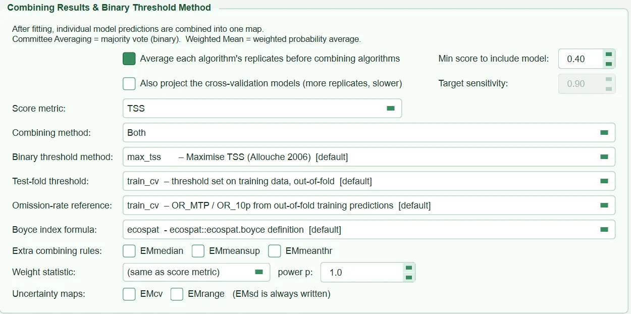
This box does two jobs: it sets the threshold of the binary map and of the threshold-dependent scores (TSS, Kappa, MCC, sensitivity, specificity, Jaccard, Sørensen, FPB), and the ensemble settings (§6.6). First the threshold and score settings:
| Name in the UI | What it does | Default | Range / options | Code |
|---|---|---|---|---|
Binary threshold method: |
Rule that converts probability to presence/absence | max_tss |
11 rules (§6.5.1) | tabs/tab_models.py:435-455 |
Target sensitivity: |
Target of the sensitivity rule |
0.90 | 0.50–1.00 | tabs/tab_models.py:456-462 |
Test-fold threshold: |
Data on which the threshold is chosen | train_cv |
train_cv / train / test |
tabs/tab_models.py:465-490 |
Omission-rate reference: |
Source of the OR_MTP and OR_10p thresholds | train_cv |
train_cv / train |
tabs/tab_models.py:491-503 |
Boyce index formula: |
Definition of the continuous Boyce index | ecospat |
ecospat / legacy |
tabs/tab_models.py:504-514 |
6.5.1 Binary threshold rule (Binary threshold method)
What it does. A threshold is chosen for each model; cells with probability equal to or greater than this threshold become 1 (sdm_core.py:7907-7915). All rules are in find_optimal_threshold (sdm_core.py:795-948). Grid-search rules try 200 equally spaced thresholds between 0.01 and 0.99.
| Rule | Threshold chosen | Source | Code |
|---|---|---|---|
max_tss |
Threshold maximizing TSS = sensitivity + specificity − 1 | Allouche et al. 2006 | sdm_core.py:891-897 |
max_kappa |
Threshold maximizing Cohen's kappa | Fielding and Bell 1997 | sdm_core.py:899-915 |
sens_spec_eq |
Minimum |sensitivity − specificity| | Liu et al. 2005 | sdm_core.py:917-931 |
p10 |
10th percentile of the presence predictions | Pearson et al. 2007 | sdm_core.py:858-864 |
min_roi |
Point on the ROC curve closest to the (0,1) corner: \min\sqrt{\mathrm{FPR}^2+(1-\mathrm{TPR})^2} | — | sdm_core.py:933-945 |
mtp |
Lowest presence prediction (no presence is left out; same as lpt) |
Pearson et al. 2007 | sdm_core.py:734-735 |
p5 |
5th percentile of the presence predictions | — | sdm_core.py:736-738 |
sensitivity |
Highest threshold retaining at least the target share of presences: the \lfloor(1-s)\,n\rfloor-th value of the sorted presence predictions | Allouche et al. 2006 | sdm_core.py:866-876 |
max_jaccard |
Maximum \mathrm{TP}/(\mathrm{TP}+\mathrm{FP}+\mathrm{FN}) | — | sdm_core.py:878-885 |
max_sorensen |
Maximum 2\mathrm{TP}/(2\mathrm{TP}+\mathrm{FP}+\mathrm{FN}) | — | sdm_core.py:878-885 |
max_fpb |
Maximum FPB = 2 × Jaccard (flexsdm's presence-background F measure) | Li and Guo 2013 | sdm_core.py:701, 878-885 |
When and how to set it. max_tss is common with pseudo-absence data and relatively independent of prevalence. In protected-area studies where a false negative is costly, p10, p5, mtp or sensitivity (e.g. 0.95) give a larger area. If omission and commission errors are equally important, sens_spec_eq is chosen. The Kappa and Jaccard family is affected by prevalence; the threshold shifts as the number of pseudo-absences changes.
Effect on results. The area in the binary maps, the range-change calculations (⑥ Range Change) and all threshold-dependent scores depend on this rule. AUC, Boyce, Brier and the calibration slope are threshold-independent. In the example run the thresholds chosen with max_tss lie between 0.06 and 0.21 (GLM_PA1 0.1294, RF_PA2 0.2058; session log): because the probability scale is low, a fixed threshold such as 0.5 would give a very narrow map with these data.
Caution. The threshold used on the map is the mean of the thresholds chosen in that model's CV folds (sdm_core.py:5852-5853); it is not re-chosen on the full-data model's own data. If the threshold cannot be computed, 0.5 is used and FAILED, 0.5 used (…) is written in the Threshold_source column (sdm_core.py:1221-1227). The Target sensitivity: box is enabled only when sensitivity is selected; the target is carried inside the key (sensitivity:0.90) and written to the run record in that form (tabs/tab_models.py:1504-1507).
6.5.2 Data on which the threshold is chosen (Test-fold threshold)
What it does. For the threshold-dependent scores in the test fold, it determines on which predictions the threshold is chosen (evaluate_all, sdm_core.py:1122-1257):
train_cv(default): the training rows are split into three inner folds (OOF_INNER_FOLDS = 3, the folds are built with the user's CV design); each row is predicted by a model that has not seen it; the threshold is chosen on these out-of-fold predictions and applied to the test fold (sdm_core.py:4876-4919,4296-4368).train: the threshold is chosen on the model's predictions for its own training rows.test: the threshold is chosen directly on the test fold, so as to maximize that fold's score (oracle threshold).
When and how to set it. train_cv is the recommended and honest option. train is cheap, but for algorithms that memorize the training data (Domain, RF, GBM, XGBoost) the threshold becomes meaningless. test is only for comparison with earlier results.
Effect on results. The test option typically gives a TSS 0.1–0.2 higher (tooltip text, tabs/tab_models.py:480-482). train_cv adds three inner fits to every CV fit; run time roughly doubles. Because the threshold on the map is the mean of the thresholds in the CV folds (§6.5.1), this choice also affects the maps.
Caution. When test is selected, an orange warning appears below the box: "Warning: 'test' picks the threshold on the very data it is scored on …" (tabs/tab_models.py:1261-1272). If the inner fit fails, the source is labelled train (inner CV unavailable) (sdm_core.py:1201-1207). ESM does not produce inner-fold predictions (sdm_core.py:4889-4890).
6.5.3 Omission-rate reference (Omission-rate reference)
What it does. OR_MTP and OR_10p are the shares of test presences falling below, respectively, the lowest and the 10th-percentile training presence prediction (sdm_core.py:1062-1115). train_cv takes these reference values from the inner out-of-fold predictions, train from the model's own training predictions.
When and how to set it. The default train_cv is recommended; it follows the same logic as ENMeval's definition of omission (Muscarella et al. 2014), with the difference that the reference is not affected by memorization.
Effect on results. It affects only the OR_MTP and OR_10p columns and the ENMeval selection rule in Tuning (§6.7); it does not affect the maps.
Caution. When train is selected, the warning is: "Warning: with in-sample references OR_10p / OR_MTP are unreliable for over-fitting algorithms …". If the threshold value is equal to or below the lowest prediction of the evaluation set, omission is 0 by construction; HABITUS flags this with the OR_10p_degenerate column and writes a note for the algorithm if this happens in at least half of the folds (sdm_core.py:1100-1114, 5787-5816).
6.5.4 Boyce index formula (Boyce index formula)
What it does. ecospat is a line-by-line port of the ecospat::ecospat.boyce function (sdm_core.py:475-543): the predictions of all evaluated rows give the expected distribution (E), the predictions of the presences give the observed distribution (P); a window whose width is 1/10 of the prediction range is moved across 101 positions, F=P_i/E_i is computed in each window, consecutive repeated F values are removed, and the index is the Spearman correlation between the window lower bounds and F (Hirzel et al. 2006; Boyce et al. 2002). legacy is the earlier HABITUS definition, computed with a fixed window of width 0.1 and 101 centres on the [0, 1] axis (sdm_core.py:612-664).
When and how to set it. ecospat (default) for results comparable with ecospat in R. legacy is only for reproducing an earlier result.
Effect on results. It changes the Boyce scores, and the ensemble selection and weights when Boyce is the score metric. A code comment records that on the same BIOCLIM predictions legacy gives 0.007 and ecospat 0.334 (sdm_core.py:560-562).
Caution. If the evaluation set contains no presences or fewer than 5 rows, Boyce is NaN (sdm_core.py:605-609).
6.6 Ensemble settings (Combining Results)
| Name in the UI | What it does | Default | Range / options | Code |
|---|---|---|---|---|
Average each algorithm's replicates before combining algorithms |
Two-level ensemble | on | on / off | tabs/tab_models.py:516-530 |
Also project the cross-validation models (more replicates, slower) |
Also projects the CV models | off | on / off | tabs/tab_models.py:532-540 |
Combining method: |
Basic ensemble rules written | Both |
Weighted Mean / Committee Averaging / Both |
tabs/tab_models.py:403-417 |
Score metric: |
Member filtering metric | TSS |
TSS / ROC / Boyce |
tabs/tab_models.py:418 |
Min score to include model: |
Minimum score | depends on metric: TSS 0.40, ROC 0.70, Boyce 0.50 | 0–1 | tabs/tab_models.py:419-433, sdm_core.py:6093 |
Extra combining rules: |
Additional rules | all off | EMmedian, EMmeansup, EMmeanthr |
tabs/tab_models.py:543-558 |
Weight statistic: |
Weighting statistic | (same as score metric) |
+ AUC, TSS, Boyce |
tabs/tab_models.py:559-566 |
power p: |
Weighting power | 1.0 | 0.5–10.0 | tabs/tab_models.py:567-575 |
Uncertainty maps: |
Additional uncertainty maps | off (EMsd always) | EMcv, EMrange |
tabs/tab_models.py:576-583 |
6.6.1 Two-level ensemble
What it does. When on (default), the replicates of the same algorithm (one full-data model per PA set; also the CV models if §6.6.2 is on) are averaged first; the mean per algorithm, the standard deviation between replicates and the vote share of the replicates are computed (EnsembleModeler.predict_by_algorithm, sdm_core.py:6234-6331). The ensemble is built from these algorithm means (sdm_core.py:6359-6376). When off, every model that passes the filter enters a single flat weighted mean (sdm_core.py:6377-6407).
When and how to set it. Leave it on: otherwise an algorithm with many replicates gets more votes in the ensemble.
Effect on results. In addition, <algo>_mean_prob, <algo>_mean_bin and, if there are several replicates, <algo>_sd maps are written for each algorithm (sdm_core.py:7964-8021). Weights are computed at the algorithm level; in the example run the TSS weights are GLM 0.271, MaxEnt 0.265, GAM 0.241, RF 0.223.
Caution. When off, EMsd is not written unless an additional uncertainty map is selected (sdm_core.py:6416-6419); the phrase (EMsd is always written) in the UI applies only to the two-level mode.
6.6.2 Also projecting the CV models
What it does. By default only the full-data models are projected (as many replicates per algorithm as there are PA sets). When the box is on, the models of the CV folds are also projected and each is written as a separate file (<algo>_PA1_RUN1_prob.tif …) (sdm_core.py:7850-7916). The choice is also passed to ⑤ Future Scenarios (tabs/tab_models.py:1538-1546).
When and how to set it. When more replicates are wanted for within-algorithm instability (SD between replicates). When the number of PA sets is 1, only one replicate per algorithm remains, so the <algo>_sd map can only be produced with this box.
Effect on results. Projection time and disk use increase roughly (folds + 1)-fold. The ensemble mean also includes the CV models.
Caution. The ensemble is built only from the projected models (sdm_core.py:6343-6355, 8028-8035). When the box is off, if only some CV models pass the minimum score and no full-data model does, the ensemble is not written and the program gives the message "No full-data model reached the minimum … Lower the minimum score, or tick 'Also project the cross-validation models' …" (sdm_core.py:8040-8054). When the box is on, each CV model is filtered separately by its own fold score; the model of a weak fold may be left out.
6.6.3 Combining method and extra rules
What it does. Combining method: determines which basic rules are computed and written: Weighted Mean → EMwmean, Committee Averaging → EMca, Both → both (tabs/tab_models.py:1670-1694; sdm_core.py:6173-6183, 6409-6412). A rule that is not selected is not computed, written or scored. Definitions (in two-level mode, \bar p_a is the algorithm mean, w_a the weight, v_a the share of the algorithm's replicates that say "present" at their own threshold):
Extra rules (sdm_core.py:6016-6040): EMmedian is the per-cell median of the member probabilities; EMmeansup is the simple mean of the "superior" members whose weight statistic is equal to or above the members' mean (flexsdm meansup); EMmeanthr is the mean probability of the members that reach their own threshold in the cell, 0 if none does (flexsdm meanthr; Velazco et al. 2022).
When and how to set it. The weighted mean and committee averaging are consensus methods that performed well in the comparison of Marmion et al. (2009). The median is robust to an extreme member; meanthr gives a broad map of the "at least one member says present" type.
Effect on results. Each rule produces separate _prob and _bin maps and receives a separate hold-out score (§6.6.6). EMca is a vote share, not a probability.
Caution. Committee averaging is unweighted across algorithms; the weight statistic affects only EMwmean and EMmeansup.
6.6.4 Score metric and minimum score
What it does. A model enters the ensemble if its Score metric: value is equal to or greater than the Min score to include model: value (EnsembleModeler._filter_models, sdm_core.py:6185-6196). The score of the full-data models is the mean of the CV folds (§6.4.6). The default minimum score depends on the metric: ROC 0.70, TSS 0.40, Boyce 0.50 (sdm_core.py:6086-6098); it follows the metric until the user types a value, and is not changed after that (tabs/tab_models.py:1696-1710).
When and how to set it. With spatially blocked CV, honest TSS values usually lie in the 0.3–0.6 range; this is why 0.40 was chosen for TSS (code comment, sdm_core.py:6086-6092). It is raised if weak models are to be excluded; set it by looking at the score of the best model so that the ensemble does not end up empty.
Effect on results. The number of ensemble members, and therefore the map, changes. In the example run all eight of the eight full-data models met the condition TSS ≥ 0.40 (Models included in combined map: 8/8).
Caution. If no model passes the threshold, the EM* maps are not written but the algorithm maps are; the status text starts with WARNING - NO COMBINED MAP: and the message states the score of the best model (sdm_core.py:6198-6232; tabs/tab_models.py:1831-1833).
6.6.5 Weight statistic, weighting power and uncertainty maps
What it does. The member weight is computed as
where s_i is the statistic selected with Weight statistic: (default: the score metric) and p the power p: value (sdm_core.py:5988-6005). Non-finite scores receive an equal share; if all weights are zero, members are weighted equally. Filtering is still done with the score metric. EMsd is the standard deviation between members (ddof = 1); EMcv = SD / mean (0 in cells where the mean ≈ 0); EMrange = maximum − minimum (sdm_core.py:6068-6083). Uncertainty surfaces are written without normalization and are never thresholded (sdm_core.py:8057-8068).
When and how to set it. p=1 is weighting proportional to the score (same meaning as power in the sdm package); 2–3 can be used to emphasize the best members. It is possible to choose a weight statistic different from the score metric, e.g. filtering with TSS and weighting with Boyce.
Effect on results. As p grows, EMwmean approaches the best algorithm. Uncertainty maps do not change the ensemble map.
Caution. Uncertainty surfaces require at least two members; in a single-algorithm run (in two-level mode) EMsd is not produced (sdm_core.py:6073-6074).
6.6.6 Binary threshold of the ensemble
The program converts the ensemble maps to binary with the following thresholds (EnsembleModeler.binary_threshold, sdm_core.py:6423-6461): for EMca 0.5 (majority vote); for EMwmean the mean of the members' thresholds weighted by the map weights; for EMmedian the median of the member thresholds; for EMmeansup the mean threshold of the superior members; for EMmeanthr the smallest member threshold (sdm_core.py:6043-6065). In the example run the EMwmean threshold is 0.1166 and the EMca threshold 0.5. Ensemble maps are not stretched to their own range; they are only clipped to [0, 1] (sdm_core.py:8074-8081).
6.6.7 Hold-out score of the ensemble and member selection from the other folds
Because the ensemble map is built from models that have seen all presences, it is not scored on its own map. Instead, for each PA set × fold group, CV models that have not seen that fold (one per algorithm) are combined with the ensemble's rule and scored only on the held-out rows of that fold; the reported value is the mean over fold groups (EnsembleModeler.evaluate_cv, sdm_core.py:6516-6696). Whether a member enters the ensemble, and its weight, are computed from the mean of the same algorithm's scores in the other folds (leave one fold out; the same fold number is also left out in the other PA sets; sdm_core.py:6463-6496). The ensemble's threshold is chosen on the training surface built from the members' inner out-of-fold training predictions (sdm_core.py:6619-6657). In the example run all eight of the eight fold groups were used; for EMwmean ROC 0.902, TSS 0.659, Boyce 0.726, and for EMca ROC 0.878, TSS 0.660, Boyce 0.725 were found. These rows are added to evaluation_scores.csv with PA_set = Ensemble, CV_run = CV_holdout, Score_source = cv_holdout (sdm_core.py:6698-6729).
Note: The hold-out score is computed with a flat (single-level) combination in each fold, because each group contains only one model per algorithm. In a single-fold design there is no "other fold", so the member is weighted by its own fold score, and this is counted in the
cv_notetext (sdm_core.py:6511-6513).
6.7 Tuning search (Tuning (optional))
Figure 6.5. The settings panel of the Tuning (optional) sub-tab (the result table and plot on the right are empty because no search has been run): for MaxEnt, rm 0.50–4.00 in steps of 0.50 and the L, LQ, H, LQH, LQHP feature classes; 40 grid points, about 160 model fits.
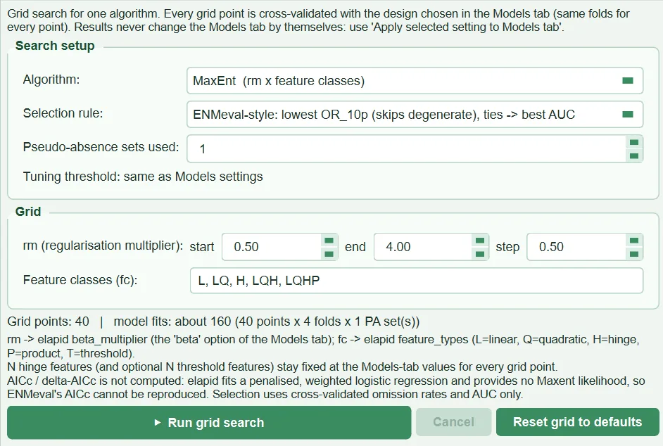
This sub-tab searches the settings of a single algorithm over a grid. Each grid point is tested with the CV design, threshold rule and source, omission reference, Boyce formula and clamping setting from Algorithm Settings, on the same folds at all points (tabs/tab_models.py:1274-1294; sdm_tuning.py:394-494). For each point only CV is run (run(cv_only=True)); the full-data model and variable importance are not computed.
| Name in the UI | What it does | Default | Range / options | Code |
|---|---|---|---|---|
Algorithm: |
Algorithm to search | MaxEnt (rm x feature classes) |
MaxEnt, GBM, RF, SVM, ANN, XGBoost, LightGBM, GLMNET, CART, GAM (those installed) | tabs/tab_tuning.py:91-96 |
Selection rule: |
Rule for choosing the best point | ENMeval-style | 3 rules | tabs/tab_tuning.py:97-110, sdm_tuning.py:84-88 |
Pseudo-absence sets used: |
First n PA sets used in scoring | 1 | 1–20 | tabs/tab_tuning.py:111-114 |
rm (regularisation multiplier): |
Sequence of MaxEnt regularization multipliers | start 0.50, end 4.00, step 0.50 | 0.05–50 | tabs/tab_tuning.py:211-226, sdm_tuning.py:506 |
Feature classes (fc): |
Sets of MaxEnt feature classes | L, LQ, H, LQH, LQHP |
letters L, Q, H, P, T | tabs/tab_tuning.py:227-233, sdm_tuning.py:505 |
| Grid rows of the other algorithms | Comma-separated list of values or start:end[:step] |
depends on algorithm (below) | — | tabs/tab_tuning.py:234-242 |
▶ Run grid search, Cancel, Reset grid to defaults |
Start; stop between points; return to defaults | — | — | tabs/tab_tuning.py:137-148 |
Apply selected setting to Models tab, Save table as CSV… |
Writes the selected point to the algorithm options; saves the table | — | — | tabs/tab_tuning.py:170-178, 480-499 |
Default grids (sdm_tuning.py:626-643, 776-793, 837-843): GBM n_estimators 20, 50, 100, 200, 500 × learning_rate 0.01, 0.1, 0.3 × min_samples_leaf 1–10, 20, 30 (flexsdm tune_gbm, 180 points); RF max_features from 2 to the number of predictors × n_estimators 200–1200 (flexsdm tune_raf); SVM C 1, 2, 4, 8, 16 × gamma 0.001, 0.01, 0.1, 0.2 (kernlab sigma = sklearn gamma); ANN hidden_layer_sizes 2, 4, 6, 8 × alpha = 2 × nnet decay; 3 × 3 × 3 for XGBoost and LightGBM; GLMNET C 0.01–10 × l1_ratio 0–1; CART max_depth × min_samples_leaf × ccp_alpha; GAM n_splines 5–20 × lam 0.1–10.
6.7.1 Selection rule (Selection rule)
What it does. enmeval: the point with the lowest mean OR_10p, ties broken by the highest mean test AUC (Muscarella et al. 2014; Kass et al. 2021). enmeval_guard: first discards points worse than one fold-SD below the best AUC, then applies the same rule. max_auc: the highest mean test AUC. Points whose OR_10p is 0 only because of tied low predictions ("degenerate") are not selected under the ENMeval rules (sdm_tuning.py:238-298). The rule can be changed after the search has finished without refitting (tabs/tab_tuning.py:415-418).
When and how to set it. For MaxEnt, ENMeval-style agrees with common practice; enmeval_guard to prevent the selection of points with markedly low AUC.
Effect on results. The selected point is written to the algorithm options with Apply selected setting to Models tab; the main run uses it. The search result, the grid, the rule and whether the selected point was actually used in the run are written to habitus_run_config.json as a tuning_<algo> section (tabs/tab_models.py:2195-2208).
Caution. AICc is not computed; the program says so with the note "AICc / delta-AICc is not computed: …" (sdm_tuning.py:62-66). Because selection is made on the same folds that produce the reported scores, the scores of the tuned algorithm are optimistic; there is no nested validation (sdm_tuning.py:68-78). Searches exceeding 60 points or 600 fits ask for confirmation (tabs/tab_tuning.py:36-38, 318-327). The result table is written automatically to the file <output>/tuning/tuning_<algo>.csv (tabs/tab_tuning.py:397-413).
6.8 Evaluation results (Evaluation Results)
Figure 6.6. The Evaluation Results sub-tab after the example run: ROC-AUC, TSS and Boyce values for each algorithm, PA set and CV run.
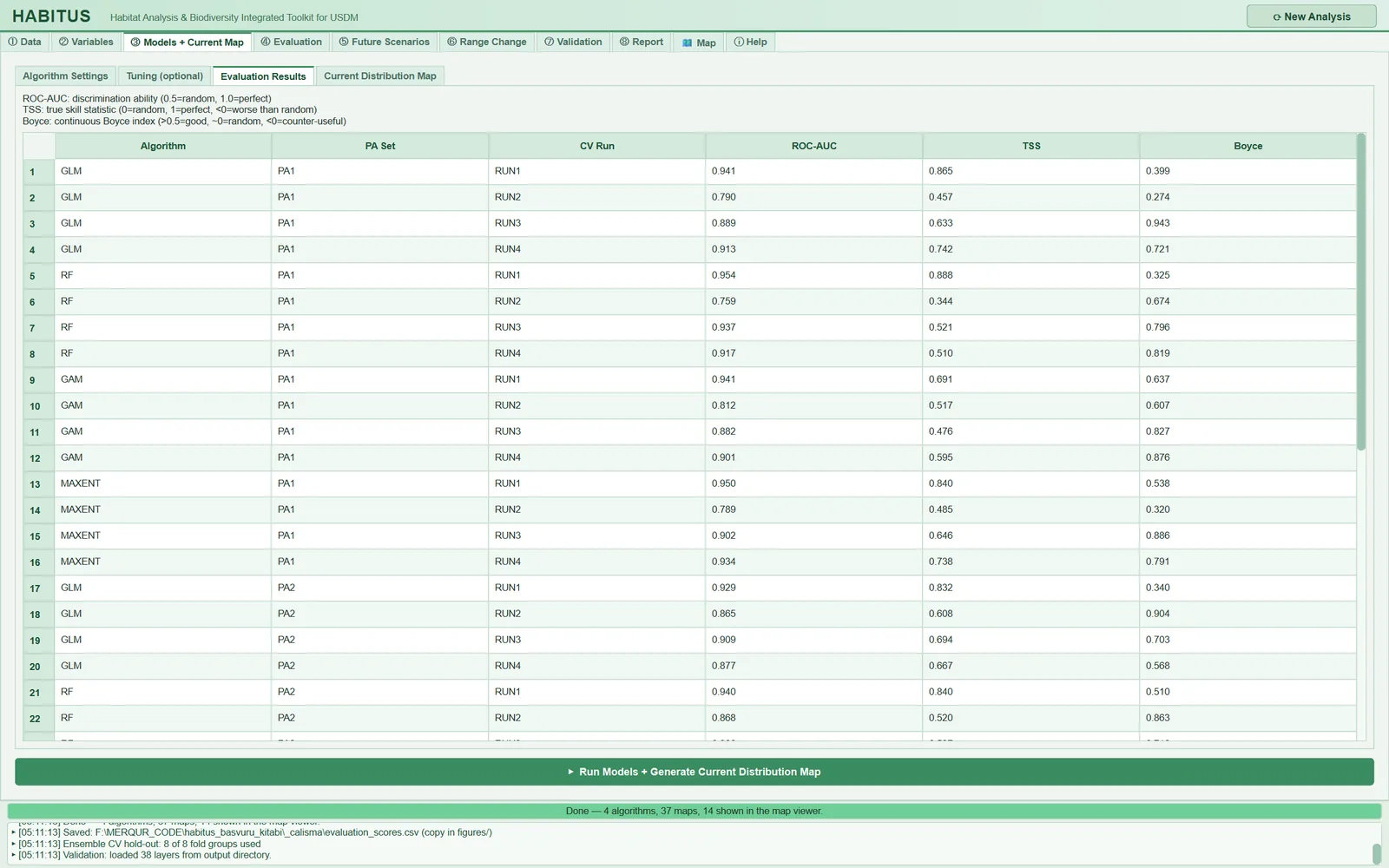
The table shows the first six columns of the evaluation_scores_table output: Algorithm, PA Set, CV Run, ROC-AUC, TSS, Boyce (tabs/tab_models.py:618-634, 1753-1782). The rows come first as CV runs (RUN1…), then the full-data models (Full, carrying the CV mean), and finally the ensemble's hold-out rows (EMwmean, EMca …, PA Set = Ensemble). Values of 0.8 and above are shown in green, 0.6–0.8 in orange, below 0.6 in red; non-numeric values appear as N/A. The tooltip of the ensemble rows says that the score comes from the CV hold-outs, not from the map (tabs/tab_models.py:1769-1774).
The full table and the other columns (threshold, prevalence, Brier, calibration slope, Kappa, MCC, sensitivity, specificity, omission rates, Threshold_source, Score_source …) are in the evaluation_scores.csv file; their meanings are explained in Chapter 7.
Tip: The colour thresholds are the same for all metrics; for Boyce, values above 0.5 are already considered good (explanation at the top of the tab). The colour is not a judgement but a marker that makes the table easier to scan.
6.9 Current distribution map (Current Distribution Map)
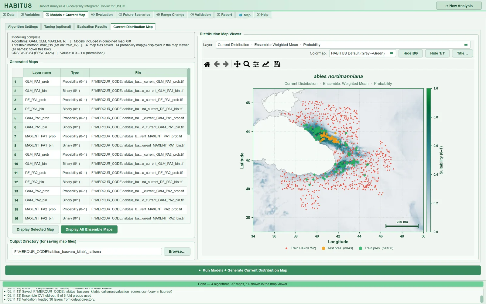
Figure 6.7. The Current Distribution Map sub-tab: on the left the status text, the Generated Maps table and the output folder; on the right the weighted-mean ensemble map, overlaid with training presences (green, n=100), test presences (orange, n=43) and training pseudo-absences (red, n=752).
| Name in the UI | What it does | Default | Code |
|---|---|---|---|
| Status text | Algorithms, number of models entering the ensemble, threshold rule and source, number of maps, CRS; the long layer list is in the tooltip | — | tabs/tab_models.py:643-651, 1817-1834 |
Generated Maps table |
Layer name, Type (Probability (0–1) / Binary (0/1)), File |
— | tabs/tab_models.py:654-666, 1798-1812 |
Display Selected Map |
Loads the map of the selected rows into the viewer | — | tabs/tab_models.py:1963-1977 |
Display All Ensemble Maps |
Loads all maps beginning with EM |
— | tabs/tab_models.py:1979-1984 |
Output Directory (for saving map files) |
Folder the maps are written to; if empty, the output folder from ① Data | from ① Data | tabs/tab_models.py:679-686, 1467-1477 |
Distribution Map Viewer |
Layer selection, colour scale, Hide BG, Hide T/T, Title… |
— | tabs/tab_models.py:688-695; map_widget.py:346-401 |
When the run finishes, all probability maps are loaded into the viewer automatically (tabs/tab_models.py:1808-1812); layer names have the form Current Distribution · <algorithm> · PA-<n> · Probability or … · Ensemble: Weighted Mean · Probability (tabs/tab_models.py:35-47). The split in the first CV fold of the first PA set is drawn over the map: training presences in green, test presences in orange, training pseudo-absences in red (tabs/tab_models.py:1859-1907; sdm_core.py:5470-5513). The same points are written to the output folder as occurrence_train.csv, occurrence_test.csv and occurrence_all_splits.csv (tabs/tab_models.py:1914-1961). Hide BG hides the pseudo-absence points, Hide T/T the training/test points; the viewer's other tools are described in Chapter 12.
Caution. In the example run the status text says 37 map files saved. 14 probability map(s) displayed: 8 individual models × 2 (probability, binary) + 4 algorithms × 3 (mean probability, mean binary, SD) + 2 ensembles × 2 + EMsd + 4 novelty layers (NT1, NT2, MIC_NT1, MIC_NT2) = 37 files; the 14 maps loaded into the viewer are the 8 individual maps ending in _prob, the 4 algorithm means and the 2 ensemble maps. The "test" points on the map do not come from an 80/20 split but from the first spatial fold; this is why they form a contiguous cluster (the orange cluster in Figure 6.7). The values are raw probabilities clipped to [0, 1]; the word normalised in the status text does not mean that the map has been stretched to its own range (sdm_core.py:7884-7889).
6.10 Outputs and what passes to the next step
To the <output>/current/ folder (tabs/tab_models.py:1615; sdm_core.py:7895-8103):
<species>_current_<ALGO>_PA<n>_prob.tifand_bin.tif: each full-data model (_PA<n>_RUN<k>_…if the CV models are projected).<species>_current_<ALGO>_mean_prob.tif,_mean_bin.tif,<ALGO>_sd.tif: algorithm means and spreads (in two-level mode).<species>_current_EMwmean_prob.tif,EMca_…, the extra rules andEMsd.tif/EMcv.tif/EMrange.tif.NT1,NT2,MIC_*novelty (ExDet) layers andprojection_options.json(Chapter 8).
In the output root: evaluation_scores.csv (and a copy in figures/), habitus_run_config.json (CV design, block size per fold, SSB, fold sizes, threshold settings, ensemble members and weights, hold-out ensemble scores), occurrence_*.csv and, if searches were run, tuning/tuning_<algo>.csv (tabs/tab_models.py:2056-2240).
What passes to the next tabs: the models and the ensemble object, the ensemble rules and weights, the two-level mode and the projected replicates (⑤ Future Scenarios uses the same rules, tabs/tab_models.py:1539-1546), the thresholds (⑥ Range Change), the map files (the ⑦ Validation layer lists are filled automatically, tabs/tab_models.py:1853-1857).
6.11 Expert questions
Q1. How is the spatial block size determined; is it the same as blockCV?
Answer: No; it follows the same logic but is simplified. For each predictor at the presence points, HABITUS builds an omnidirectional empirical variogram with 15 classes, takes the median of the outer third of the classes as the sill, takes the distance at which 95% of the sill is first reached as the range, and uses the median across predictors as the block size (sdm_spatial.py:166-281). blockCV instead samples from raster cells or points and estimates the range by fitting a variogram model (Valavi et al. 2019). In HABITUS no variogram model is fitted and the value derives only from the predictor values at the presence points; the result may differ from blockCV. If a comparable value is wanted, the range found in blockCV should be entered manually in the Block size: field.
Q2. What happens if the block design cannot build enough blocks; do the scores silently revert to a random split?
Answer: First the block is halved up to six times and this is noted; if there are still not as many blocks as the requested folds, or fewer than two folds contain both classes, the program falls back to random folds, flags degraded, the note starts with WARNING (design not applied):, and [BLOCKING FAILED - scores are optimistic] is added to the run summary (sdm_spatial.py:454-495; sdm_core.py:5135-5140, 5933-5934). There is no silent fallback; however, the user needs to read the log or the report.
Q3. Does the full-data model that draws the map have an independent score?
Answer: It does not, and cannot; it is fitted on all the data. The program writes into the Full row the mean of the CV fold scores of the same algorithm and PA set (and the mean of the fold thresholds), Score_source = cv_mean (sdm_core.py:5818-5853). It is also this mean that selects and weights the ensemble members. This is similar to the "score of the full model = summary of the CV scores" approach in biomod2.
Q4. Is the binary threshold chosen on the test data? Are the threshold-dependent scores optimistic?
Answer: Not with the default train_cv: the threshold is chosen on the three-inner-fold out-of-fold predictions of the training rows and applied to the test fold (sdm_core.py:4876-4927, 1193-1220). The test option optimizes the threshold on the test fold; the code and tooltip state that this typically inflates TSS by 0.1–0.2. This difference matters when comparing with workflows in R that search for the threshold on the evaluation data, such as ecospat.max.tss or biomod2: HABITUS's default TSS may come out systematically lower than theirs.
Q5. Is the ensemble score computed from the ensemble's own map?
Answer: No. In each PA × fold group, CV models that have not seen that fold are combined with the ensemble rule and scored only on that fold; member selection and weights come from the scores of the other folds (leave one fold out) (sdm_core.py:6463-6696). The resubstitution score from the map (evaluate) does not enter this table at all (sdm_core.py:6698-6706). This design also brings the selection and weighting step of the ensemble inside the validation; it is more conservative than biomod2's ensemble evaluation.
Q6. Why is there a two-level ensemble; how does it differ from biomod2's EMwmean?
Answer: In biomod2, each individual model (PA × run) enters the ensemble as a separate member. HABITUS by default first averages the replicates of an algorithm, then weights the algorithms (sdm_core.py:6109-6132, 6359-6376). In this way an algorithm with many replicates does not dominate, and within-algorithm instability becomes visible in a separate SD map. If the box is unticked, the flat combination is restored; this option can be used for comparison with biomod2, but biomod2's weight definition (including the rank-based decay) is not identical.
Q7. How are the weights computed; what happens to a negative score?
Answer: w_i=\max(s_i,0)^p/\sum_j\max(s_j,0)^p; negative scores are set to 0, non-finite ones receive an equal share, and if all weights are zero equal weights are given (sdm_core.py:5988-6005). In the example run the TSS means are 0.687 (GLM), 0.566 (RF), 0.611 (GAM), 0.672 (MaxEnt), while the weights are 0.271/0.223/0.241/0.265; that is, at p=1 the weights are close to one another. If more discrimination is wanted, p is increased.
Q8. How is SSB computed, and is it the same as dismo::ssb?
Answer: For each fold, the distances of the test presences and test absences to the nearest training presence are taken, pooled and put in a ratio (sdm_spatial.py:808-881). dismo::ssb also divides the test-presence→training-presence distance by the test-background→training-presence distance (Hijmans 2012); HABITUS uses the pseudo-absences in the test fold as background and draws a seeded subsample when there are more than 3000 points. The interpretation thresholds (0.7 and 1.3) are specific to HABITUS and are not a published cut-off.
Q9. Are the scores optimistic after a tuning search? Is nested validation performed?
Answer: Yes, they are optimistic; no nested validation is performed. The best point is chosen on the same folds that produce the reported scores; the program writes this to the log and the UI with SELECTION_BIAS_NOTE and states that the size of the optimism is not measured (sdm_tuning.py:68-78; tabs/tab_tuning.py:396). The user can partly remove this bias by testing the tuned algorithm with an independent test set (External test points (CSV)) or with the independent map in ⑦ Validation.
Q10. Why is ENMeval's delta-AICc criterion absent?
Answer: elapid fits MaxEnt as a penalized, weighted logistic regression and does not provide the Maxent likelihood; HABITUS therefore does not compute AICc at all rather than approximating it (sdm_tuning.py:38-46, 62-66). Selection rests on out-of-fold omission and AUC (the complexity warning of Warren and Seifert 2011 is addressed only indirectly in this way).
Q11. With an external test CSV, is the standard deviation across RUN1…RUN4 a measure of uncertainty?
Answer: No. Each run is trained on the same full data and tested on the same test points (sdm_core.py:5417-5427); the difference comes only from the algorithm's own randomness. The program writes this as a note in the report (sdm_core.py:5341-5347). For uncertainty, the difference between PA sets or blocked CV should be used.
Q12. Which setting changes the map most?
Answer: For the probability map, the choice of algorithms and the threshold for entry into the ensemble (§6.3, §6.6.4); for the binary map and area, the threshold rule and the threshold source (§6.5.1–6.5.2), because the threshold on the map is the mean of the thresholds chosen in the CV folds. The CV design does not change the map directly, but through the scores it changes member selection, the weights and the threshold. In the example run the thresholds lie in the 0.06–0.21 range, so small differences in the threshold rule can change the area markedly; if the sensitivity to this is to be measured, the Classification Thresholds table in ④ Evaluation can be used (Chapter 7).
6.12 Common mistakes and pitfalls
- Comparing a high AUC obtained with the
randomdesign with spatially blocked results in the same table. The design is written in the_cv_strategyfield of every row and in the run record. - Keeping
Min score to include model:high, e.g. 0.7 out of AUC habit, and switching the metric to TSS: no model passes andWARNING - NO COMBINED MAP:appears. If the user has not typed a value, the default follows the metric; if they have, it does not. - Lowering
Cross-validation folds:below 4 withcheckerboard2: some of the four folds are never tested. - Expecting the scores to change by changing
Training data %:; if CV succeeds, they do not change (§6.4.6). - Reporting in a paper the TSS produced with
Test-fold threshold:=test; the UI shows an orange warning for this choice. - Taking the orange "test" points on the map for a random test set; they are the points of the first spatial fold.
- Not understanding why the ensemble is not written when
Also project the cross-validation modelsis off and only CV models pass the threshold; the message suggests ticking this box. - Looking for
EMsdin a single-algorithm run: at least two members are needed. - Starting the main run without applying the point selected in the tuning search with
Apply selected setting to Models tab; the search result does not change the settings by itself. Theselected_options_used_in_this_runfield in the run record shows this.
6.13 References
Allouche, O., Tsoar, A., Kadmon, R., 2006. Assessing the accuracy of species distribution models: prevalence, kappa and the true skill statistic (TSS). Journal of Applied Ecology 43, 1223–1232. https://doi.org/10.1111/j.1365-2664.2006.01214.x
Araújo, M.B., New, M., 2007. Ensemble forecasting of species distributions. Trends in Ecology & Evolution 22, 42–47. https://doi.org/10.1016/j.tree.2006.09.010
Boyce, M.S., Vernier, P.R., Nielsen, S.E., Schmiegelow, F.K.A., 2002. Evaluating resource selection functions. Ecological Modelling 157, 281–300. https://doi.org/10.1016/S0304-3800(02)00200-4
Fielding, A.H., Bell, J.F., 1997. A review of methods for the assessment of prediction errors in conservation presence/absence models. Environmental Conservation 24, 38–49. https://doi.org/10.1017/S0376892997000088
Hijmans, R.J., 2012. Cross-validation of species distribution models: removing spatial sorting bias and calibration with a null model. Ecology 93, 679–688. https://doi.org/10.1890/11-0826.1
Hirzel, A.H., Le Lay, G., Helfer, V., Randin, C., Guisan, A., 2006. Evaluating the ability of habitat suitability models to predict species presences. Ecological Modelling 199, 142–152. https://doi.org/10.1016/j.ecolmodel.2006.05.017
Kass, J.M., Muscarella, R., Galante, P.J., Bohl, C.L., Pinilla-Buitrago, G.E., Boria, R.A., Soley-Guardia, M., Anderson, R.P., 2021. ENMeval 2.0: Redesigned for customizable and reproducible modeling of species' niches and distributions. Methods in Ecology and Evolution 12, 1602–1608. https://doi.org/10.1111/2041-210X.13628
Li, W., Guo, Q., 2013. How to assess the prediction accuracy of species presence–absence models without absence data? Ecography 36, 788–799. https://doi.org/10.1111/j.1600-0587.2013.07585.x
Liu, C., Berry, P.M., Dawson, T.P., Pearson, R.G., 2005. Selecting thresholds of occurrence in the prediction of species distributions. Ecography 28, 385–393. https://doi.org/10.1111/j.0906-7590.2005.03957.x
Marmion, M., Parviainen, M., Luoto, M., Heikkinen, R.K., Thuiller, W., 2009. Evaluation of consensus methods in predictive species distribution modelling. Diversity and Distributions 15, 59–69. https://doi.org/10.1111/j.1472-4642.2008.00491.x
Muscarella, R., Galante, P.J., Soley-Guardia, M., Boria, R.A., Kass, J.M., Uriarte, M., Anderson, R.P., 2014. ENMeval: An R package for conducting spatially independent evaluations and estimating optimal model complexity for Maxent ecological niche models. Methods in Ecology and Evolution 5, 1198–1205. https://doi.org/10.1111/2041-210X.12261
Pearson, R.G., Raxworthy, C.J., Nakamura, M., Peterson, A.T., 2007. Predicting species distributions from small numbers of occurrence records: a test case using cryptic geckos in Madagascar. Journal of Biogeography 34, 102–117. https://doi.org/10.1111/j.1365-2699.2006.01594.x
Roberts, D.R., Bahn, V., Ciuti, S., Boyce, M.S., Elith, J., Guillera-Arroita, G., Hauenstein, S., Lahoz-Monfort, J.J., Schröder, B., Thuiller, W., Warton, D.I., Wintle, B.A., Hartig, F., Dormann, C.F., 2017. Cross-validation strategies for data with temporal, spatial, hierarchical, or phylogenetic structure. Ecography 40, 913–929. https://doi.org/10.1111/ecog.02881
Valavi, R., Elith, J., Lahoz-Monfort, J.J., Guillera-Arroita, G., 2019. blockCV: An R package for generating spatially or environmentally separated folds for k-fold cross-validation of species distribution models. Methods in Ecology and Evolution 10, 225–232. https://doi.org/10.1111/2041-210X.13107
Velazco, S.J.E., Rose, M.B., de Andrade, A.F.A., Minoli, I., Franklin, J., 2022. flexsdm: An R package for supporting a comprehensive and flexible species distribution modelling workflow. Methods in Ecology and Evolution 13, 1661–1669. https://doi.org/10.1111/2041-210X.13874
Warren, D.L., Seifert, S.N., 2011. Ecological niche modeling in Maxent: the importance of model complexity and the performance of model selection criteria. Ecological Applications 21, 335–342. https://doi.org/10.1890/10-1171.1