5. Models I: algorithms and their settings (③ Models → Algorithm Settings)
Tab: ③ Models + Current Map → Algorithm Settings · Code: tabs/tab_models.py (UI), sdm_core.py build_model, SDMModeler (computation), sdm_niche.py (BIOCLIM, Domain, ESM), sdm_tuning.py (tunable parameters)
5.1 What this tab does
The Algorithm Settings sub-tab answers the "with which method" question of modelling. Here you tick which of the 18 algorithms will be run and enter the settings (hyperparameters) of each. A hyperparameter is a setting that the model does not learn from the data but that the user fixes in advance: the number of trees, a penalty coefficient, the number of layers and so on.
Its place in the workflow is as follows:
- Input: the pseudo-absence datasets produced by the ① Data tab (presence + pseudo-absence rows for each replicate), the MaxEnt background, the optional presence-only background, and the predictors (continuous and categorical) selected in the ② Variables tab. Until these two steps are complete, the run button gives the message "Complete ① Data and ② Variables steps first." (
tabs/tab_models.py:1394-1395). - Processing: when the
▶ Run Models + Generate Current Distribution Mapbutton is pressed, every ticked algorithm is trained on every pseudo-absence set, in the cross-validation folds and with the full data (sdm_core.py:5352SDMModeler.run). The settings on this page are collected by_collect_algo_optsand passed toSDMModelerasalgo_options(tabs/tab_models.py:1142-1209,1569-1573). - Output: the trained models, evaluation scores, variable importances and the current distribution map. These are shown in the
Evaluation ResultsandCurrent Distribution Mapsub-tabs and in the ④ Evaluation tab. All settings used are written to thesettings.models.algorithm_optionsfield of thehabitus_run_config.jsonfile.
The cross-validation design, threshold and ensemble settings are in the lower half of the same page; they are described in Chapter 6. This chapter covers only the choice of algorithms and the algorithm settings.
5.2 Screen layout

The page consists of four areas:
Select Algorithms(top left): 18 check boxes, nine in each of two columns (tabs/tab_models.py:125-150). See §5.3.Algorithm Options(top right): one tab per algorithm. Because the tab bar cannot fit all 18 tabs, it is scrolled with the arrow buttons on the right (tabs/tab_models.py:173-194). Pages with six or more rows (BRT, XGBoost, LightGBM, CatBoost, MaxEnt, ESM) are laid out in two columns (tabs/tab_models.py:197-201). Each tab is described in its own subsection in §5.6–§5.23.Training SettingsandCombining Results & Binary Threshold Method(lower half): Chapter 6.- Run button:
▶ Run Models + Generate Current Distribution Map.
The data of the example run are Abies nordmanniana (626 records; 143 presences after thinning; WorldClim 2.1 bioclimatic variables, 2.5′; 8 variables selected in ② Variables: bio_2, bio_3, bio_8, bio_9, bio_11, bio_15, bio_18, bio_19; 2 pseudo-absence sets × 1000 points; MaxEnt background 10,000 points; seed 42). The numbers in this chapter are taken from the habitus_run_config.json, evaluation_scores.csv and session log of this run.
5.3 Algorithm selection (Select Algorithms)
| Name in the UI | What it does | Default | Range / options | Code |
|---|---|---|---|---|
GLM – Generalised Linear Model |
Logistic regression | on | on / off | tabs/tab_models.py:129 |
RF – Random Forest |
Random forest | on | on / off | tabs/tab_models.py:132 |
The other 16 boxes (GBM, BRT, SVM, ANN, XGBoost, LightGBM, CatBoost, GAM, MaxEnt, ENFA, Mahalanobis, BIOCLIM, Domain, GLMNET, CART, ESM) |
Runs the corresponding algorithm | off | on / off | tabs/tab_models.py:130-146 |
When the program starts, only GLM and RF are ticked. If the package required by an algorithm is not installed, its box is unticked and disabled, [not installed] is appended to its name and the installation command is shown in the tooltip (e.g. "Not installed — pip install pygam"; tabs/tab_models.py:152-168). Algorithms that need a package: XGBoost (xgboost), LightGBM (lightgbm), CatBoost (catboost), GAM (pygam), MaxEnt (elapid); the other 13 algorithms run with scikit-learn or numpy (sdm_core.py:127-146). If no box is ticked, the run stops with the message "Select at least one algorithm." (tabs/tab_models.py:1397-1400).
Note: The order in which algorithms are ticked or predictors are added does not change the result. In every run the columns are ordered first continuous, then categorical, and each group in natural name order (
sdm_core.py:3892-3899).
5.4 Rules common to all algorithms
5.4.1 Which rows are used for training: presence-absence and presence-only
In HABITUS the algorithms fall into three groups according to the rows they use in training:
- Presence–pseudo-absence (classifier) models: GLM, GLMNET, GAM, GBM, BRT, RF, CART, SVM, ANN, XGBoost, LightGBM, CatBoost and the GLM/RF-based ESM. They use all rows of the pseudo-absence set (presence = 1, pseudo-absence = 0) (
sdm_core.py:4480-4498). - Presence + background: MaxEnt. It uses the presences in the training fold and the MaxEnt background sampled separately in ① Data; pseudo-absences do not enter MaxEnt training (
sdm_core.py:4595-4603,tabs/tab_models.py:1580). ENFA also uses the presence-only background, if available, to estimate the global environmental distribution (sdm_core.py:4079-4092). - Presence only: Mahalanobis, BIOCLIM and Domain are fitted from presence rows only (
sdm_core.py:4227-4228,4281-4282).
Evaluation, however, is the same whatever the group: AUC, TSS, Boyce and the others are computed from the presences and pseudo-absences in the test fold. For presence-only methods, if no presence is left in the test fold, about one fifth of the presences in the training fold are moved to the test set (sdm_core.py:5455-5468; for the full model 5686-5696).
5.4.2 Scaling of the input
For scale-sensitive methods, standardisation (mean 0, standard deviation 1) is done inside the program, learned from the training rows only; the user does not need to scale beforehand:
- GLM and GLMNET: the terms (linear, quadratic, interaction) are generated first, then these terms are standardised (
sdm_core.py:3488-3505). - SVM and ANN: the predictors are standardised (
sdm_core.py:3562-3581). - Tree methods (GBM, BRT, RF, CART, XGBoost, LightGBM, CatBoost) are unaffected by scale; no scaling is done.
- MaxEnt features are generated by elapid's transformer. GAM, ENFA, Mahalanobis, BIOCLIM and Domain work with raw values; ENFA and Mahalanobis remove scale themselves through the covariance matrix, BIOCLIM through percentiles, and Domain through differences divided by the presence range.
5.4.3 Categorical variables
Categorical rasters (land cover, aspect class and the like) reach the model as integer class codes; each algorithm uses them as follows:
| Algorithm | Handling of the categorical variable | Code |
|---|---|---|
| GLM, GLMNET, SVM, ANN | One 0/1 column (one-hot) for each class seen in training; the codes are not squared, scaled or multiplied. A class not seen in training gets 0 in all columns of that variable | sdm_core.py:3364-3443 |
| GAM | Factor term f(), one coefficient per class; a single-class variable is skipped; the effect of an unseen class is taken as 0 |
sdm_core.py:3320-3361, 4525-4549 |
| MaxEnt | elapid's categorical feature class (one-hot, penalised with beta_categorical); unseen class 0 |
sdm_core.py:4606-4612, 4712-4718, 4760-4770 |
| GBM, BRT, RF, CART, XGBoost, LightGBM, CatBoost | The integer code is split like a numeric column | sdm_core.py:3476-3479 |
| ENFA, Mahalanobis, BIOCLIM, Domain | Categorical variables are left out; "… is an envelope/distance model for continuous predictors: the categorical variable(s) … are excluded from it." is written to the log | sdm_core.py:4010-4036 |
| ESM | Categorical variables do not enter the pairs | sdm_core.py:4389-4393 |
Caution: In tree methods the class code is split like an ordered number: codes 3 and 4 are treated as "close" and 3 and 12 as "far". If the order of the codes carries no ecological meaning, the tree can separate the classes only with several splits. CatBoost's own categorical handling is not used in HABITUS.
5.4.4 Reproducibility and the random seed
Every learner that involves randomness (RF, GBM, BRT, CART, SVM, ANN, GLMNET, XGBoost, LightGBM, CatBoost, MaxEnt, ESM folds) is seeded with the Random seed in ① Data (default 42) (sdm_core.py:115-124, 3474-3475, 4643). Two runs with the same data, the same settings and the same seed produce the same models. Permutation importance is also computed with a generator specific to the (PA set, fold, algorithm) triple but derived from the seed (sdm_core.py:4847-4853). The seed used is in the random_seed field of habitus_run_config.json.
5.4.5 Class balance and clamping (two settings from Training Settings)
Balance classes (weight presences vs pseudo-absences) and Clamp predictors to the training range when predicting are in the Training Settings group and are described in Chapter 6; but because they behave differently depending on the algorithm, they are summarised here. When balancing is on (default off), each algorithm takes its class weight as follows (sdm_core.py:3670-3716):
| Algorithm | Form of balancing |
|---|---|
| GLM, RF, SVM, GLMNET, CART, LightGBM | class_weight='balanced' |
| CatBoost | auto_class_weights='Balanced' |
| GBM, BRT | balanced sample weights (sample_weight) |
| XGBoost | scale_pos_weight = number of pseudo-absences / number of presences |
| ANN | balanced sample weights (if the installed scikit-learn supports this) |
| ESM | only in the GLM- or RF-based small models |
| GAM, MaxEnt, ENFA, Mahalanobis, BIOCLIM, Domain | not supported; the setting has no effect for these algorithms |
When clamping is on, before every prediction the predictors are clamped to the min–max range of all pseudo-absence sets; in addition, elapid's clamp=True setting is passed explicitly to MaxEnt (sdm_core.py:4650-4655, 4929-4962).
5.4.6 Relation to the tuning sub-tab
The Tuning (optional) sub-tab tries the parameters of some algorithms with a cross-validated grid search and writes the selected value to this page with Apply selected setting. The parameters that can be written to this page (tabs/tab_models.py:1212-1229, 1231-1259) and the default grids of the tuning tab (sdm_tuning.py) are:
| Algorithm | Parameters written to this page | Default grid (source) |
|---|---|---|
| MaxEnt | Feature types, Regularisation multiplier (β / RM) |
rm 0.5–4.0 step 0.5; fc L, LQ, H, LQH, LQHP (sdm_tuning.py:502-552) |
| GBM | n_estimators, learning_rate, subsample, min_samples_leaf, max_depth |
flexsdm tune_gbm: trees 20–500, learning rate 0.01/0.1/0.3, leaf 1–10, 20, 30 (sdm_tuning.py:626-630) |
| RF | n_estimators, min_samples_leaf, max_features |
flexsdm tune_raf: mtry 2…number of predictors, ntree 200–1200 (sdm_tuning.py:633-634, 787-793) |
| SVM | C, gamma |
flexsdm tune_svm: C 1–16, sigma 0.001–0.2 → gamma the same value (sdm_tuning.py:636-637, 654-675) |
| ANN | alpha (L2), Hidden layers |
flexsdm tune_net: single layer 2–8 neurons, decay 0.01–10 → alpha = 2 × decay (sdm_tuning.py:639-640, 678-689) |
| XGBoost | n_estimators, max_depth, learning_rate |
HABITUS's grid: 100/300/500; 3/6/9; 0.01/0.05/0.1 (sdm_tuning.py:779-781) |
| LightGBM | n_estimators, num_leaves, learning_rate |
HABITUS's grid: 100/300/500; 15/31/63; 0.01/0.05/0.1 (sdm_tuning.py:782-784) |
| GLMNET | C (inverse penalty), l1_ratio (alpha) |
C 0.01/0.1/1/10; l1_ratio 0–1 step 0.25 (sdm_tuning.py:837-838) |
| CART | max_depth, min_samples_leaf, ccp_alpha |
2/3/5/8; 1/5/10/20; 0/0.002/0.01 (sdm_tuning.py:839-841) |
| GAM | n_splines, lam (smoothing) |
5/10/15/20; 0.1/0.6/2/10 (sdm_tuning.py:842-843) |
GLM, BRT, CatBoost, ENFA, Mahalanobis, BIOCLIM, Domain and ESM are not in the tuning tab; their values are entered only on this page. The tuning search itself is described in Chapter 6.
5.5 Guide to choosing algorithms
The table below is a starting guide derived from the structure seen in the code and from the example run; it does not say that one method will be better than another on every dataset. The numbers in the "Speed" column are the time taken by the 4 cross-validation folds of one pseudo-absence set in the example run (including inner folds; from the log).
| Algorithm | Data type | Speed | Interpretability | Tendency to overfit (with defaults) | When |
|---|---|---|---|---|---|
| GLM | presence–pseudo-absence | very fast (0.7 s) | high (coefficients) | low–medium (L2-penalised, quadratic) | baseline model in every study |
| GLMNET | presence–pseudo-absence | fast | high | low (elastic net) | many predictors, few records |
| GAM | presence–pseudo-absence | medium (10 s) | high (response curves) | medium | non-linear, smooth responses |
| MaxEnt | presence + background | slow (165 s) | medium–high | depends on β and feature classes | presence-only data, comparability |
| RF | presence–pseudo-absence | medium (21 s) | low | high training fit (training AUC 1.000) | many records, complex interactions |
| GBM | presence–pseudo-absence | medium | low–medium | low (stumps) | flexible additive model |
| BRT | presence–pseudo-absence | medium–slow | low–medium | medium | boosting along the lines of Elith et al. (2008) |
| XGBoost, LightGBM, CatBoost | presence–pseudo-absence | fast–medium | low | high (deep trees) | many records (hundreds), comparison |
| CART | presence–pseudo-absence | very fast | very high (single tree) | unstable, stepped surface | explanatory purposes |
| SVM | presence–pseudo-absence | slows as n grows | low | depends on C and gamma | comparison |
| ANN | presence–pseudo-absence | medium | very low | high (100+50 neurons) | many records |
| ENFA | presence + background | very fast | medium (axes) | low | presence-only, coarse niche |
| Mahalanobis | presence only | very fast | medium | low | elliptical niche assumption |
| BIOCLIM | presence only | very fast | very high | low; sensitive to extreme records | climate envelope, comparison |
| Domain | presence only | fast (grows with number of presences) | high | low; sensitive to single records | similarity-based comparison |
| ESM | presence–pseudo-absence (pairs) | grows with number of pairs | medium | low (bivariate models) | very few records (about < 30) |
In the example run (143 presences, 8 variables) the cross-validation means of the four algorithms were: GLM AUC 0.889, TSS 0.687, Boyce 0.607; MaxEnt 0.895, 0.672, 0.605; RF 0.892, 0.566, 0.677; GAM 0.872, 0.611, 0.653. The difference between training and test AUC (dAUC) is 0.031 for GLM, 0.055 for MaxEnt, 0.087 for GAM and 0.108 for RF; RF fits the training data most tightly.
Tip: Instead of looking for a single "best" algorithm, it is common practice to run several algorithms from different families (a regression, a tree ensemble, MaxEnt) and combine them in an ensemble map; combining is in Chapter 6.
5.6 GLM: generalised linear model

Family and implementation. Binary (logistic) regression: the logit of the probability of presence is a linear combination of the predictors. It is fitted with scikit-learn LogisticRegression (solver lbfgs, at most 2000 iterations) inside a pipeline that first generates terms and then standardises them (sdm_core.py:3481-3492). Data type presence–pseudo-absence. The penalty is an L2 (ridge) penalty applied to the coefficients of the standardised terms.
| Name in the UI | What it does | Default | Range / options | Code |
|---|---|---|---|---|
Model terms: |
Which terms enter the model | quadratic |
linear, quadratic, interactions |
tabs/tab_models.py:721-735; sdm_core.py:3300-3317 |
Regularisation C: |
Inverse penalty strength (L2) | 1.00 | 0.001 – 1 000 000 | tabs/tab_models.py:736-745; sdm_core.py:3482 |
5.6.1 Model terms
- What it does.
lineargenerates only the x term for each predictor,quadraticthe x and x^2 terms, andinteractionsin addition all pairwise products (x_i x_j) (sdm_core.py:3300-3317). Compared with MaxEnt feature classes they are L, LQ and LQP respectively. With p predictors the number of terms is p, 2p and p + p(p+1)/2; with 8 predictors 8, 16 and 44. - When and how to set it.
quadraticallows a unimodal (optimum) response along a variable; it is the classical assumption of the ecological niche and suits most studies.lineargives only monotonically increasing or decreasing responses; it is chosen with very few records or to keep interpretation simple.interactionsneeds at least a few hundred presence records; by the ten-events-per-variable rule in the tooltip, about 440 records with 8 predictors. - Effect on results. As terms increase, training fit increases, response curves bend and the risk of going beyond the calibration range (extrapolation) in projections grows; a squared term gives a curve that falls or rises steeply outside the range.
- Caution. Terms are not applied to the codes of categorical variables; they are applied only to continuous variables (
sdm_core.py:3364-3378).
5.6.2 Regularisation C
- What it does. The objective function of scikit-learn is C\sum_i \ell_i + \tfrac{1}{2}\lVert\beta\rVert^2: as C decreases the penalty grows and the coefficients are pulled towards zero. Because the penalty is applied to standardised terms, it affects all terms equally.
- When and how to set it. If the number of terms is large relative to the number of records (
interactions, many predictors), C is reduced (0.1 or 0.01). R'sglm()is unpenalised (as are the GLMs of biomod2, sdm and flexsdm); to reproduce their results, enter C = 1e6 (tooltip,tabs/tab_models.py:741-743). - Effect on results. Because the penalty is defined relative to a sum of losses, its relative effect decreases as the number of rows increases: in the example run a training fold has about 860 rows (three quarters of 1143 rows) and C = 1 is a light penalty. The tooltip reports that in a Pinus brutia example the default penalty raised the cross-validation AUC from 0.804 (unpenalised) to 0.824.
- Caution. GLM is not in the tuning tab; if a search over C is wanted, GLMNET (l1_ratio = 0), which carries the same penalty family, can be used.
Equivalence with R. With Model terms = linear and C = 1e6 the model solves the same objective function as glm(y ~ x1 + x2 + …, family = binomial) in R; for quadratic the corresponding form is y ~ x + I(x^2). biomod2's GLM eliminates terms by AIC-based stepwise selection; HABITUS has no stepwise selection, it has a penalty instead.
5.7 GBM: gradient boosting (scikit-learn)
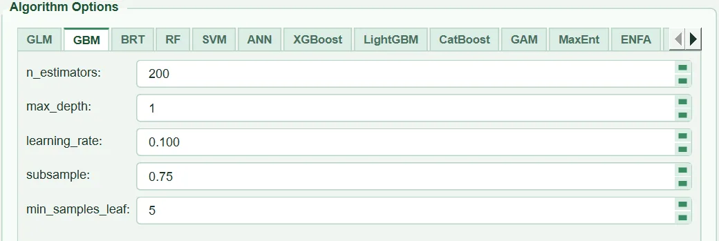
Family and implementation. Gradient-boosted decision trees (boosting): each new tree corrects the error (the gradient of the log-loss) of the sum of the previous trees. scikit-learn GradientBoostingClassifier (sdm_core.py:3516-3529). Presence–pseudo-absence. No scaling needed. GBM and BRT use the same implementation; only their defaults and ranges differ.
| Name in the UI | What it does | Default | Range / options | Code |
|---|---|---|---|---|
n_estimators: |
Number of trees | 200 | 10 – 5000 (step 100) | tabs/tab_models.py:750; sdm_core.py:3524 |
max_depth: |
Tree depth (gbm: interaction.depth) |
1 | 1 – 10 | tabs/tab_models.py:751-752; sdm_core.py:3525 |
learning_rate: |
Coefficient that shrinks the contribution of each tree (gbm: shrinkage) |
0.100 | 0.001 – 1.0 | tabs/tab_models.py:753; sdm_core.py:3526 |
subsample: |
Fraction of rows drawn for each tree (gbm: bag.fraction) |
0.75 | 0.1 – 1.0 (step 0.05) | tabs/tab_models.py:756-758; sdm_core.py:3527 |
min_samples_leaf: |
Minimum rows in a leaf (gbm: n.minobsinnode) |
5 | 1 – 200 | tabs/tab_models.py:754-755; sdm_core.py:3528 |
5.7.1 n_estimators and learning_rate
- What it does. The model has the form F = \sum_{m=1}^{M} \nu\, h_m(x); M is the number of trees and \nu the learning rate. Together they determine the model's total "amount of learning".
- When and how to set it. If the learning rate is reduced, the number of trees must be increased proportionally for the same fit (0.1 → 0.01 means about 10 times as many trees). Elith et al. (2008) recommend a learning rate that reaches at least 1000 trees. The best pair can be searched with the flexsdm grid in the
Tuning (optional)tab. - Effect on results. Many trees + a high rate lead to overfitting, few trees + a low rate to underfitting. Run time increases linearly with the number of trees.
- Caution. The number of trees is not selected automatically by cross-validation (there is no early stopping as in dismo's
gbm.step); the number entered is used as is.
5.7.2 max_depth
- What it does. The depth of each tree. 1 means a single-split tree (a "stump") and the model becomes an additive function of the predictors with no interactions. 2 and above allow variable interactions.
- When and how to set it. The default 1 is close to the
interaction.depth= 1 default of flexsdmfit_gbm(sdm_core.py:3517-3522). If interactions are thought to be important and the number of records is high, 2–3 are tried. - Effect on results. According to the tooltip, stumps prevent the surface from collapsing to zero in most cells and give a higher Boyce at the same AUC (
tabs/tab_models.py:752). - Caution. gbm's
interaction.depthand scikit-learn'smax_depthdefine the same tree at 1; at larger values the two packages grow trees differently, so the numbers do not map one to one.
5.7.3 subsample
- What it does. Each tree is built with a random subset of the training rows of this fraction (stochastic gradient boosting).
- When and how to set it. The range 0.5–0.75 is common; 1.0 uses all rows and removes the randomness.
- Effect on results. Values below 1 reduce variance and overfitting; the result becomes dependent on the seed (it remains reproducible because the seed is fixed).
- Caution. Very small values can leave some trees almost without presences in data with few presences.
5.7.4 min_samples_leaf
- What it does. The minimum number of rows a leaf may hold; splits that would create smaller leaves are not made.
- When and how to set it. The default 5 corresponds to gbm's
n.minobsinnodedefault. With noisy data or few records it can be raised to 10–20. - Effect on results. As it grows, the trees become coarser, the surface smoother and overfitting smaller.
- Caution. With
max_depth= 1 each tree has only one split, so its effect is limited.
5.8 BRT: boosted regression trees
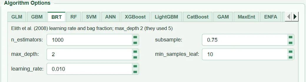
Family and implementation. The same method and the same scikit-learn class as GBM (GradientBoostingClassifier), but with defaults chosen according to the guide of Elith et al. (2008): a low learning rate, many trees, 75% bagging (sdm_core.py:3530-3548). Presence–pseudo-absence.
| Name in the UI | What it does | Default | Range / options | Code |
|---|---|---|---|---|
n_estimators: |
Number of trees | 1000 | 100 – 10 000 (step 100) | tabs/tab_models.py:765; sdm_core.py:3543 |
max_depth: |
Tree depth (Elith et al.: tree.complexity) |
2 | 1 – 10 | tabs/tab_models.py:766-767; sdm_core.py:3544 |
learning_rate: |
Learning rate | 0.010 | 0.001 – 0.5 | tabs/tab_models.py:768; sdm_core.py:3545 |
subsample: |
Bagging fraction (bag.fraction) |
0.75 | 0.1 – 1.0 | tabs/tab_models.py:769; sdm_core.py:3546 |
min_samples_leaf: |
Minimum rows in a leaf | 10 | 1 – 100 | tabs/tab_models.py:770; sdm_core.py:3547 |
5.8.1 max_depth
- What it does. Tree complexity; it determines the level of interaction.
- When and how to set it. Elith et al. (2008) used
tree.complexity= 5 in their examples. HABITUS takes 2 as the default; according to the code comment, on presence–pseudo-absence data deep trees push the suitability of most cells to zero and halve the Boyce index (sdm_core.py:3532-3537). For the original setting, enter 5. - Effect on results. As depth increases, interaction and training fit increase and the suitability surface becomes sharper.
- Caution. With greater depth, fewer trees are needed for the same fit; it should be considered together with
n_estimators.
5.8.2 n_estimators, learning_rate, subsample, min_samples_leaf
- What it does. The same as in GBM (§5.7).
- When and how to set it. Elith et al. (2008) recommend choosing the learning rate so that at least 1000 trees are formed; the default 0.01 and 1000 trees follow this rule.
subsample0.75 is the bagging fraction recommended by the authors. - Effect on results. If the learning rate is lowered from 0.01 to 0.005 and the number of trees raised to 2000, the model is usually similar but smoother; run time doubles.
- Caution. dismo
gbm.stepselects the number of trees itself by 10-fold cross-validation; in HABITUS the number of trees is fixed and BRT is not in the tuning tab. A user who wants to choose the number of trees from the data can search GBM in the tuning tab and use the same values here.
5.9 RF: random forest
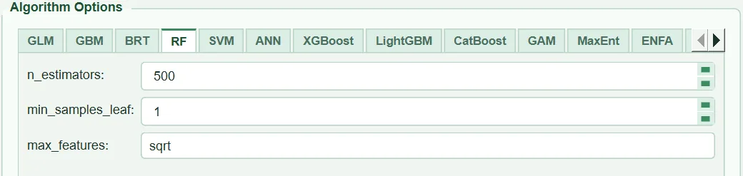
Family and implementation. An ensemble of bagged (bootstrap) classification trees; at each split a random subset of the predictors is tried (Breiman 2001). scikit-learn RandomForestClassifier; tree depth unlimited, all processor cores used (sdm_core.py:3549-3561). Suitability is the mean of the leaf proportions of the trees. Presence–pseudo-absence.
| Name in the UI | What it does | Default | Range / options | Code |
|---|---|---|---|---|
n_estimators: |
Number of trees (randomForest: ntree) |
500 | 50 – 2000 (step 100) | tabs/tab_models.py:778; sdm_core.py:3555 |
min_samples_leaf: |
Minimum rows in a leaf (randomForest: nodesize) |
1 | 1 – 50 | tabs/tab_models.py:779; sdm_core.py:3557 |
max_features: |
Number of predictors tried at each split (randomForest: mtry) |
sqrt |
sqrt, log2, integer, fraction between 0 and 1 |
tabs/tab_models.py:780-783, 1160-1172; sdm_core.py:3558 |
5.9.1 n_estimators
- What it does. The number of trees in the forest.
- When and how to set it. The code comment notes the recommendation of Oshiro et al. (2012) of at least 128 trees and that 500 is stable on most SDM data (
sdm_core.py:3550-3553). 500 is sufficient in most cases; if the map looks noisy, it is raised to 1000. - Effect on results. The number of trees does not create overfitting; it only reduces random fluctuation of the prediction. Time and memory increase linearly (in the example run 4 folds 21 s).
- Caution. Increasing the number of trees does not change RF's tight fit to the training data (training AUC 1.000 in the example run); leaf size is used for that.
5.9.2 min_samples_leaf
- What it does. The minimum number of rows in a leaf; 1 means the trees are fully grown (the randomForest classification default is
nodesize= 1). - When and how to set it. If the training–test AUC difference is large or the map looks patchy, it is raised to 5–10.
- Effect on results. As it grows, the probability surface becomes smoother, training AUC falls and overfitting decreases.
- Caution. A very large value forces presences into the same leaf as pseudo-absences in data with few presences and lowers discriminatory power.
5.9.3 max_features
- What it does. The number of candidate predictors chosen at random at each split.
sqrt= \lfloor\sqrt{p}\rfloor (2 with 8 predictors),log2= \lfloor\log_2 p\rfloor, integer = that many predictors, a number between 0 and 1 = that fraction of the predictors. - When and how to set it.
sqrtis the value Breiman recommended for classification and the defaultmtryof R randomForest. The tuning tab, like flexsdm, tries from 2 up to the number of predictors. - Effect on results. A small value makes the trees differ from each other (reduces their correlation); a large value lets strong predictors dominate in every tree.
- Caution. An unreadable entry stops the run with the message "RF max_features: '…' is not sqrt, log2, a whole number of variables or a fraction between 0 and 1."; zero or negative values are also rejected (
tabs/tab_models.py:1160-1172). Entering 1 means "1 predictor", not "100%".
Equivalence with R. The defaults are the same as the R randomForest(…, ntree = 500, mtry = floor(sqrt(p)), nodesize = 1) classification. Difference: randomForest computes probability from the proportion of tree votes, scikit-learn from the mean of leaf proportions; with leaf size 1 the two are very close. The down-sampled RF recommended by Valavi et al. (2021) is not available in HABITUS; Balance classes applies weighting, not down-sampling.
5.10 SVM: support vector machine
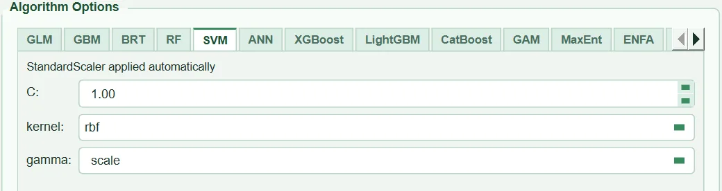
Family and implementation. Kernel-based margin classifier. scikit-learn SVC with probability=True: probabilities are obtained by Platt scaling in scikit-learn's own internal cross-validation (sdm_core.py:3562-3568). Predictors are standardised, categoricals are one-hot encoded. Presence–pseudo-absence.
| Name in the UI | What it does | Default | Range / options | Code |
|---|---|---|---|---|
C: |
Error penalty; smaller gives a smoother boundary | 1.00 | 0.001 – 1000 | tabs/tab_models.py:789; sdm_core.py:3565 |
kernel: |
Kernel function | rbf |
rbf, linear, poly, sigmoid |
tabs/tab_models.py:790 |
gamma: |
Kernel width (RBF, poly, sigmoid) | scale |
scale, auto or a number |
tabs/tab_models.py:791-793, 1156-1159 |
5.10.1 C
- What it does. The penalty for misclassified training points. A large C gives a complex boundary that fits the training data tightly, a small C a smoother boundary.
- When and how to set it. flexsdm
tune_svmtries the range 1–16; the tuning tab uses the same grid. - Effect on results. As C grows, training AUC rises and overfitting increases.
- Caution. SVM run time grows roughly on a quadratic-to-cubic scale with the number of rows; it is slow with tens of thousands of pseudo-absences.
5.10.2 kernel and gamma
- What it does. The RBF kernel is k(x,x') = \exp(-\gamma\lVert x-x'\rVert^2); \gamma determines the radius of influence of a training point.
scale= 1/(p\cdot \mathrm{Var}(X)),auto= 1/p. Because the predictors are standardised, the two give the same value with continuous variables; they differ if one-hot columns are present. - When and how to set it. RBF is sufficient for most SDMs. A number can also be typed in the box; the tuning tab writes a number here. flexsdm's kernlab
sigmahas the same definition as scikit-learn'sgamma, no conversion is needed (sdm_tuning.py:654-675). - Effect on results. A large \gamma gives a narrow area of influence and a patchy, overfitted surface; a small \gamma gives a smooth, nearly linear surface. With the
linearkernelgammahas no effect. - Caution. Because Platt scaling uses its own internal cross-validation, the probability ranking may not be exactly the same as the
decision_functionranking; this is documented scikit-learn behaviour.
5.11 ANN: artificial neural network (multilayer perceptron)
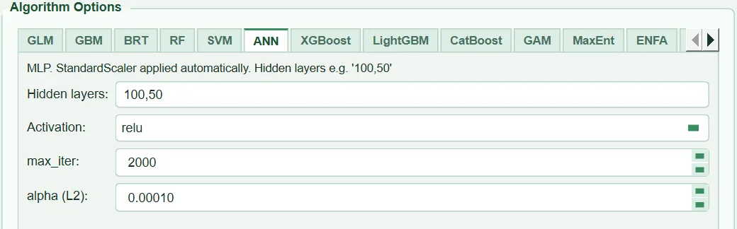
Family and implementation. Feed-forward neural network. scikit-learn MLPClassifier (Adam optimiser, the scikit-learn default); predictors are standardised, categoricals are one-hot encoded (sdm_core.py:3569-3581). Presence–pseudo-absence.
| Name in the UI | What it does | Default | Range / options | Code |
|---|---|---|---|---|
Hidden layers: |
Numbers of neurons in the hidden layers, comma-separated | 100,50 |
list of positive integers | tabs/tab_models.py:799, 1144-1154 |
Activation: |
Activation function | relu |
relu, tanh, logistic |
tabs/tab_models.py:800 |
max_iter: |
Maximum training iterations (epochs) | 2000 | 100 – 5000 | tabs/tab_models.py:801 |
alpha (L2): |
L2 penalty on the weights | 0.00010 | 0.0 – 100.0 | tabs/tab_models.py:802-804; sdm_core.py:3579 |
5.11.1 Hidden layers
- What it does.
100,50means two hidden layers (100 and 50 neurons);5means 5 neurons in a single layer. - When and how to set it. The default network carries thousands of weights; it is large for typical SDM data with one or two hundred presences. R nnet (biomod2, flexsdm) uses a single hidden layer and a few neurons; flexsdm
tune_nettries 2–8 neurons. With few records a single layer and 4–8 neurons are recommended. - Effect on results. As neurons increase, flexibility and overfitting increase and run time lengthens.
- Caution. An unreadable entry stops the run with the message "ANN hidden layers: '…' is not a list of positive whole numbers separated by commas (e.g. 100, 50)." (
tabs/tab_models.py:1144-1154).
5.11.2 alpha (L2)
- What it does. A penalty on the squares of the weights (weight decay).
- When and how to set it. nnet's
decayparameter corresponds to \alpha = 2\timesdecay(tooltip andsdm_tuning.py:678-689; this relation is derived from the two objective functions and has not been tested numerically against R nnet). The decay range 0.01–10 of the flexsdm grid corresponds to alpha 0.02–20; the default 0.0001 is much smaller than these. - Effect on results. As it grows, the surface becomes smoother and overfitting decreases.
- Caution. A large network + a small alpha is the setting that overfits most easily.
5.11.3 Activation and max_iter
- What it does.
reluproduces a piecewise linear response,tanhandlogisticsmooth S-shaped responses.max_iteris the maximum number of epochs of the optimiser. - When and how to set it. nnet uses
logisticactivation; for comparison with R,logisticcan be chosen. If a convergence warning appears,max_iteris increased. - Effect on results.
relugives angular transitions in response curves,logistic/tanhsmoother curves. - Caution. Early stopping is not used; the network is trained up to
max_iteror scikit-learn's convergence criterion.
5.12 XGBoost: extreme gradient boosting
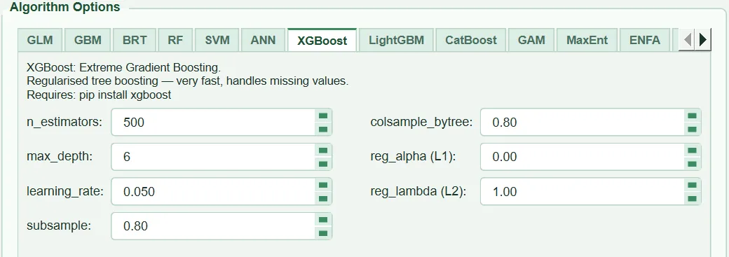
Family and implementation. Regularised gradient-boosted trees (Chen and Guestrin 2016), xgboost.XGBClassifier, loss function log-loss (sdm_core.py:3582-3608). Presence–pseudo-absence. Two settings not in the UI are fixed: min_child_weight = 1, gamma = 0.
| Name in the UI | What it does | Default | Range / options | Code |
|---|---|---|---|---|
n_estimators: |
Number of boosting rounds (trees) | 500 | 50 – 5000 | tabs/tab_models.py:815 |
max_depth: |
Tree depth | 6 | 1 – 12 | tabs/tab_models.py:816 |
learning_rate: |
Learning rate (eta) | 0.050 | 0.001 – 0.5 | tabs/tab_models.py:817 |
subsample: |
Row fraction per tree | 0.80 | 0.1 – 1.0 | tabs/tab_models.py:818 |
colsample_bytree: |
Predictor fraction per tree | 0.80 | 0.1 – 1.0 | tabs/tab_models.py:819 |
reg_alpha (L1): |
L1 penalty on leaf weights | 0.00 | 0 – 10 | tabs/tab_models.py:820 |
reg_lambda (L2): |
L2 penalty on leaf weights | 1.00 | 0 – 10 | tabs/tab_models.py:821 |
5.12.1 n_estimators, learning_rate, max_depth
- What it does. Number of trees, learning rate and depth as in GBM.
- When and how to set it. The default depth of 6 is very deep compared with GBM (1) and BRT (2) and allows a high level of interaction; with a few hundred presences 2–3 is safer. The grid of the tuning tab is depth 3/6/9, rate 0.01/0.05/0.1, rounds 100/300/500.
- Effect on results. As depth and rounds increase, training fit and overfitting increase.
- Caution. There is no early stopping; the number of rounds is fixed.
5.12.2 subsample and colsample_bytree
- What it does. Each tree is built with a random subset of the rows and predictors of these fractions.
- When and how to set it. The range 0.5–0.9 is common; with few predictors (e.g. 4), if
colsample_bytreeis reduced some trees never see an important variable. - Effect on results. Small fractions reduce variance and overfitting.
- Caution. The result depends on the seed; it is reproducible because the seed is fixed.
5.12.3 reg_alpha and reg_lambda
- What it does. L1 and L2 penalties on leaf values; they shrink leaf predictions.
- When and how to set it. The defaults are XGBoost's own defaults (0 and 1). If overfitting is seen,
reg_lambdacan be raised to 5–10. - Effect on results. As the penalty increases, the probability surface is compressed towards 0.5 and becomes smoother.
- Caution. The UI note says that XGBoost can handle missing values; in HABITUS, rows with missing values are already removed in data preparation, so this feature is not used.
5.13 LightGBM: light gradient boosting
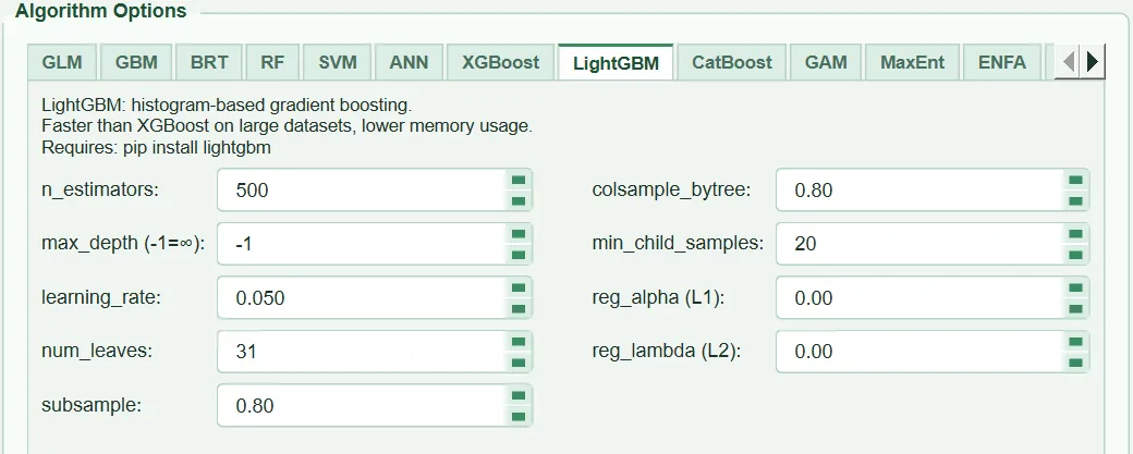
Family and implementation. Histogram-based gradient boosting with leaf-wise growth; lightgbm.LGBMClassifier (sdm_core.py:3610-3628). Tree size is controlled by the number of leaves, not by depth. Presence–pseudo-absence.
| Name in the UI | What it does | Default | Range / options | Code |
|---|---|---|---|---|
n_estimators: |
Number of rounds | 500 | 50 – 5000 | tabs/tab_models.py:837 |
max_depth (-1=∞): |
Depth limit | -1 (unlimited) | -1 – 100 | tabs/tab_models.py:838 |
learning_rate: |
Learning rate | 0.050 | 0.001 – 0.5 | tabs/tab_models.py:839 |
num_leaves: |
Maximum leaves per tree | 31 | 2 – 255 | tabs/tab_models.py:840 |
subsample: |
Row subsampling fraction | 0.80 | 0.1 – 1.0 | tabs/tab_models.py:841 |
colsample_bytree: |
Predictor fraction per tree | 0.80 | 0.1 – 1.0 | tabs/tab_models.py:842 |
min_child_samples: |
Minimum rows in a leaf | 20 | 1 – 200 | tabs/tab_models.py:843 |
reg_alpha (L1): |
L1 penalty | 0.00 | 0 – 10 | tabs/tab_models.py:844 |
reg_lambda (L2): |
L2 penalty | 0.00 | 0 – 10 | tabs/tab_models.py:845 |
5.13.1 num_leaves and max_depth
- What it does.
num_leavesdirectly limits the complexity of the tree;max_depth= -1 leaves depth unlimited. - When and how to set it. 31 leaves is more complex than a balanced tree of depth 5; with few records 7–15 leaves and
max_depth3–4 are more suitable. The tuning tab tries 15/31/63. - Effect on results. As leaves increase, interaction and overfitting increase.
- Caution. Leaf-wise growth can produce very deep, narrow branches with little data; limiting with
max_depthprevents this.
5.13.2 min_child_samples
- What it does. The minimum number of rows that must be in a leaf.
- When and how to set it. Default 20; with fewer than 50 presences it can make it hard to form leaves containing presences and can be lowered to 5–10.
- Effect on results. As it grows, the model becomes coarser.
- Caution. With very few presences the model may find no split at all and give an almost constant prediction.
5.13.3 subsample and colsample_bytree
- What it does. Row and predictor subsampling fractions.
- When and how to set it.
colsample_bytreeis applied in each tree. - Effect on results. As
colsample_bytreedecreases, the trees become more diverse. - Caution. In LightGBM, row subsampling (
subsample) is active only whensubsample_freqis greater than zero; because HABITUS does not pass this setting (sdm_core.py:3613-3628), thesubsamplevalue is not reflected in the result.
5.13.4 n_estimators, learning_rate, reg_alpha, reg_lambda
- What it does. The same meanings as in XGBoost (§5.12).
- When and how to set it. LightGBM's own default penalties are zero; in case of overfitting
reg_lambdais increased. - Effect on results. See §5.12.
- Caution. There is no early stopping.
5.14 CatBoost: categorical boosting
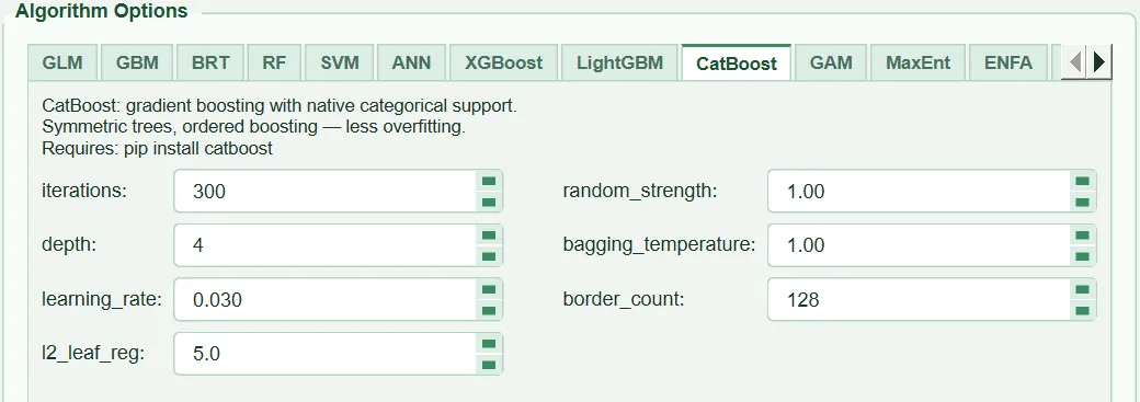
Family and implementation. Ordered boosting with symmetric trees (using the same split at each level); catboost.CatBoostClassifier (sdm_core.py:3630-3647). Presence–pseudo-absence.
| Name in the UI | What it does | Default | Range / options | Code |
|---|---|---|---|---|
iterations: |
Number of rounds | 300 | 50 – 5000 | tabs/tab_models.py:863 |
depth: |
Symmetric tree depth | 4 | 1 – 16 | tabs/tab_models.py:864 |
learning_rate: |
Learning rate | 0.030 | 0.001 – 0.5 | tabs/tab_models.py:865 |
l2_leaf_reg: |
L2 penalty on leaf values | 5.0 | 0 – 20 | tabs/tab_models.py:866 |
random_strength: |
Noise added to split scores | 1.00 | 0.01 – 10 | tabs/tab_models.py:867 |
bagging_temperature: |
Strength of the Bayesian bootstrap weights | 1.00 | 0 – 10 | tabs/tab_models.py:868 |
border_count: |
Number of split borders for continuous predictors | 128 | 1 – 255 | tabs/tab_models.py:869 |
5.14.1 iterations, learning_rate, depth
- What it does. Number of rounds, learning rate and tree depth. In a symmetric tree, depth d means exactly 2^d leaves (4 → 16 leaves).
- When and how to set it. The defaults (300 rounds, 0.03, depth 4) are a smaller model than CatBoost's library defaults (1000 rounds, depth 6). CatBoost is not in the tuning tab; values are tried by hand.
- Effect on results. As depth and rounds increase, training fit increases.
- Caution. Rate and number of rounds should be considered together (§5.7.1).
5.14.2 l2_leaf_reg, random_strength, bagging_temperature
- What it does.
l2_leaf_regshrinks leaf values;random_strengthadds randomness to split selection;bagging_temperaturedetermines the randomness of the row weights (0 = all rows equally weighted). - When and how to set it. In case of overfitting
l2_leaf_regis increased (CatBoost's own default is 3, HABITUS uses 5). - Effect on results. As all three grow, the model becomes smoother and its sensitivity to the seed increases.
- Caution.
bagging_temperature= 0 does not remove randomness;random_strengthis still in effect.
5.14.3 border_count
- What it does. Into how many possible split points (quantile borders) each continuous predictor is divided.
- When and how to set it. 128 is sufficient resolution for most bioclimatic variables.
- Effect on results. A small value makes response curves stepped; a large value lengthens run time.
- Caution. In HABITUS, categorical variables are not declared to CatBoost as categorical; the integer code is split with these borders like a continuous column (§5.4.3). The "native categorical support" in the UI note is therefore not used in HABITUS.
5.15 GAM: generalised additive model
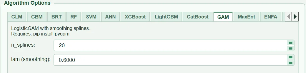
Family and implementation. Logistic additive model: the logit is the sum of a smooth (spline) function of each predictor (Hastie and Tibshirani 1986). pygam LogisticGAM; each continuous predictor is given a penalised B-spline term s() and each categorical predictor a factor term f(); there are no interaction terms (sdm_core.py:4500-4549). Presence–pseudo-absence. Works with raw values.
| Name in the UI | What it does | Default | Range / options | Code |
|---|---|---|---|---|
n_splines: |
Number of spline basis functions per predictor | 20 | 4 – 100 | tabs/tab_models.py:881-886; sdm_core.py:4508-4512 |
lam (smoothing): |
Smoothing penalty | 0.6000 | 0.0001 – 1000 | tabs/tab_models.py:887-892; sdm_core.py:4513-4514 |
5.15.1 n_splines
- What it does. The number of basis functions from which each response curve is built; it determines the maximum flexibility of the curve. Because the spline order is 3, it must be greater than 3; otherwise the message "GAM n_splines must exceed the spline order (3)." is given.
- When and how to set it. 20 is pygam's default. With few records 5–10 is sufficient and means fewer parameters; the tuning tab tries 5/10/15/20.
- Effect on results. As it increases, the curves can become more wiggly (to the extent the penalty allows); run time increases.
- Caution. The same value is applied to all predictors.
5.15.2 lam (smoothing penalty)
- What it does. The penalty coefficient applied to the second derivative (curvature) of the curve. A large
lambrings the curve closer to a straight line. - When and how to set it. 0.6 is pygam's default. If the response curves are wavy and not ecologically plausible, it is raised to 2–10; the tuning tab tries 0.1/0.6/2/10.
- Effect on results. In the example run (with defaults) the training–test AUC difference of GAM is 0.087; almost three times that of GLM (0.031). This indicates that smoothing remains light on these data.
- Caution. The penalty is not selected automatically from the data; the
lamentered is used as a fixed value.
Equivalence with R. The GAMs of biomod2 and flexsdm use mgcv; mgcv estimates the smoothing parameter from the data (GCV/REML) and its default basis is the thin plate regression spline. The pygam model in HABITUS works with a fixed lam; the response curves of the two programs can therefore differ in smoothness on the same data.
Caution: GAM does not support class balancing;
Balance classesdoes not affect GAM (sdm_core.py:3681).
5.16 MaxEnt: maximum entropy
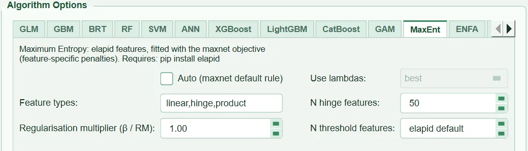
Family and implementation. Presence + background method (Phillips et al. 2006, 2017). "Features" (linear, quadratic, product, hinge, threshold) are derived from the predictors and an L1-penalised model determines which features remain. HABITUS generates the features with the elapid library (Anderson 2023) and estimates the coefficients by solving the objective function of R maxnet (sdm_core.py:3776-3836, 4551-4757). The output is elapid's cloglog transformation and is not rescaled afterwards (sdm_core.py:4772-4845).
| Name in the UI | What it does | Default | Range / options | Code |
|---|---|---|---|---|
Auto (maxnet default rule) |
Selects feature classes from the number of presences | off | on / off | tabs/tab_models.py:1056-1063; sdm_core.py:3758-3773 |
Feature types: |
Feature classes, comma-separated | linear,hinge,product |
linear, quadratic, hinge, product, threshold |
tabs/tab_models.py:1048-1055; sdm_core.py:4616-4624 |
Regularisation multiplier (β / RM): |
Regularisation multiplier | 1.00 | 0.1 – 20.0 (step 0.5) | tabs/tab_models.py:1064-1077; sdm_core.py:4625 |
Use lambdas: |
Not used (disabled) | best |
best, last |
tabs/tab_models.py:1078-1085 |
N hinge features: |
Number of hinge knots per predictor | 50 | 10 – 200 | tabs/tab_models.py:1086; sdm_core.py:4626 |
N threshold features: |
Number of threshold features per predictor | elapid default (0 = elapid's 10) |
0 – 200 | tabs/tab_models.py:1087-1091; sdm_core.py:4645-4649 |
5.16.1 The maxnet objective function is applied exactly
Because there is no Python counterpart of R glmnet in HABITUS builds, elapid on its own falls back to a scikit-learn logistic regression with a single penalty coefficient. On this path there are no feature-specific penalties and the regularisation multiplier barely changes the model (sdm_core.py:3780-3787). HABITUS therefore uses the feature transformer built by elapid but re-estimates the coefficients with the maxnet_refit function (sdm_core.py:4719-4746). maxnet solves glmnet along a λ path with standardize = FALSE, per-feature penalty factors and weights w_i = p_i + 100(1-p_i) (presence 1, background 100) and keeps the last λ. The problem solved at this last λ is, up to a constant factor (sdm_core.py:3789-3797):
Here \ell_i is the logistic loss and r_j the regularisation value of feature j; n_{\text{pres}} is the number of presences. r_j is computed with elapid's compute_regularization function according to the feature class, the number of presences, the distribution of the feature among the presences and the β multiplier (sdm_core.py:3810-3816). The intercept is unpenalised. The problem is solved with liblinear, with the features divided by n_{\text{pres}}\cdot r_j; then the MaxEnt normalisation constants (alpha, entropy) are recomputed from the background rows (sdm_core.py:3817-3835). In the run record this solver is written as "maxnet objective (feature-specific L1 penalties, last lambda)" (sdm_core.py:4743-4744).
Presences are added to the background. As with maxnet's addsamplestobackground = TRUE and Maxent's default behaviour, every presence whose predictor values are not found among the background rows is also added to the background (sdm_core.py:4698-4707). The number added is written to the maxent_settings_used.presences_added_to_background field in habitus_run_config.json; in the full model of the example run it is 91.
Automated test against R maxnet. tests/test_maxent_maxnet.py compares HABITUS's cloglog prediction with R maxnet 0.1.4 output on a subset of the data of Rutrough et al. (2019) (302 presences, 2000 background rows; ppt, silt, slope). Three settings are tested (LQH β=3, LQH β=1, LQPH β=3); in each, the Pearson and Spearman correlations are expected to exceed 0.995 and the mean absolute difference to be below 0.02 (tests/test_maxent_maxnet.py:39-50). Two additional tests check that the number of non-zero coefficients decreases as β grows (53-59) and that presences are added to the background (62-64). The R output is a file stored with the test; the test itself does not run R. The code comment reports agreement with R maxnet of Schoener D = 0.998 on the same data (sdm_core.py:3799-3800).
5.16.2 Feature types and Auto (maxnet default rule)
- What it does. Determines which feature classes are generated:
linear,quadratic,product(pairwise product),hinge(a piecewise function that increases or decreases linearly after a knot),threshold(a step). IfAutois ticked, the classes are selected for each fit from the number of training presences by the maxnet rule: fewer than 10 presences L; 10–14 LQ; 15–79 LQH; 80 and above LQHP. The threshold class is never used in the automatic rule; while the box is ticked, the text box is ignored and disabled. - When and how to set it. With few records
linearorlinear,quadraticis a defensible choice (tooltip). Merow et al. (2013) recommend choosing complexity according to the question and the data. For a search as in ENMeval/Wallace, the tuning tab tries the sets L, LQ, H, LQH, LQHP. - Effect on results. Few classes give smooth and transferable responses; many classes (especially hinge and threshold) give stepped responses that fit the calibration data tightly. With
Autoon, the cross-validation folds and the full model may use different class sets depending on their numbers of presences (sdm_core.py:4619-4622); the rule used is written to the record. - Caution. The default
linear,hinge,productis not the same as the maxnet rule (there is no quadratic class). If a comparison with maxnet is to be made,Autoshould be ticked.
5.16.3 Regularisation multiplier (β / RM)
- What it does. The coefficient that multiplies all r_j values. As it grows, the L1 penalty increases and fewer features remain non-zero.
- When and how to set it. The maxnet and Maxent default is 1. There is no single correct value; ENMeval (Muscarella et al. 2014) and kuenm therefore search for the multiplier. The tuning tab crosses rm 0.5–4.0 (step 0.5) with the feature sets and writes the selected value here. The best value depends on the calibration area; if the area changes it should be searched again (tooltip).
- Effect on results. That the number of non-zero coefficients decreases when β is raised from 1 to 6 is checked by a test (
tests/test_maxent_maxnet.py:53-59). On the map, a large β gives broader and softer suitability, a small β narrower and patchier suitability. - Caution. The effect of the value is meaningful only with the maxnet objective function; HABITUS uses this path in every fit and writes to the record that it was used.
5.16.4 N hinge features and N threshold features
- What it does. The number of hinge knots and threshold features to be generated per predictor.
- When and how to set it. 50 hinges is maxnet's default. The number of thresholds is used only if the
thresholdclass is selected; 0 leaves elapid's own value (10). - Effect on results. As the number of knots increases, the response curve can capture finer detail; the penalty limits this.
- Caution. In the tuning tab these two values are held fixed for all grid points (
sdm_tuning.py:550-551).
5.16.5 Use lambdas
The box is disabled and does not affect the result: the model is fitted at the last value of the λ path, as in maxnet (tabs/tab_models.py:1079-1085). The value is nevertheless written to the record (use_lambdas).
Note: In MaxEnt cross-validation the background is not split into folds; every fold is trained with the same background. Test scores are computed with the presences and pseudo-absences in the test fold. The size and sampling scheme of the background are set in ① Data (Chapter 3). If the installed elapid does not recognise a setting, the setting is not silently dropped; the warning "MaxEnt: the installed elapid (…) has no setting for …" is given (
sdm_core.py:4684-4691).
5.17 ENFA: ecological niche factor analysis
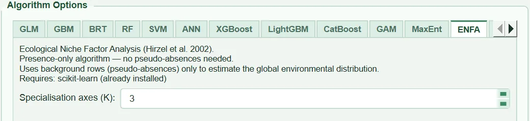
Family and implementation. A multivariate niche method that compares the environment used by the species with the general (global) environment (Hirzel et al. 2002). In HABITUS it is written with numpy (sdm_core.py:4046-4204):
- The global mean and covariance are estimated from the presence-only background in ① Data if available, otherwise from all rows of the training fold (presence + pseudo-absence); the covariance is computed with Ledoit–Wolf shrinkage and 1e-6 is added to its diagonal.
- The data are whitened with the global covariance; the marginality axis is the direction of the difference between the species mean and the global mean.
- In the subspace orthogonal to marginality, an eigendecomposition of the covariance of the presences is performed and the K axes with the largest eigenvalues are kept.
- The raw score is \exp\{-\tfrac12[d_m^2 + \sum_k (z_k-\mu_k)^2/\lambda_k]\}; d_m is the distance to the species mean along the marginality axis.
- During fitting, the score is scaled to 0–1 with the score range of the training rows; this range is stored with the model, so the same cell gets the same value in every prediction (
sdm_core.py:3719-3743,4158-4162).
Categorical variables are left out. At least 2 presences are needed.
| Name in the UI | What it does | Default | Range / options | Code |
|---|---|---|---|---|
Specialisation axes (K): |
Number of specialisation axes to keep | 3 | 1 – 10 | tabs/tab_models.py:1102-1104; sdm_core.py:4074, 4133 |
5.17.1 Specialisation axes (K)
- What it does. Determines how many additional axes enter the score besides the marginality axis. It is limited to one less than the number of predictors (
sdm_core.py:4133). - When and how to set it. 2–4 axes carry most of the variance in most cases; with few predictors (e.g. 4) K can be at most 3.
- Effect on results. As K increases, the score measures distance in more dimensions and the suitable area narrows.
- Caution. ENFA takes no other settings apart from class weighting and clamping; scale and regularisation constants are fixed in the code.
Comparison with R. adehabitatHS enfa computes the marginality and specialisation axes; for the suitability map, the original work of Hirzel et al. uses a separate computation. HABITUS's ENFA score is the Gaussian-shaped distance above; there is no numerical comparison test against R implementations.
5.18 Mahalanobis distance
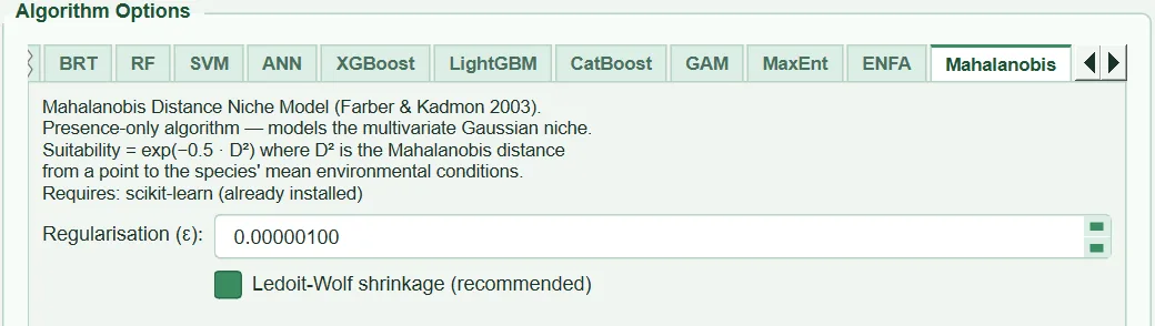
Family and implementation. Presence-only distance method: the Mahalanobis distance D^2(x) = (x-\mu)^\top \Sigma^{-1}(x-\mu) to the mean environment of the presences is computed and the raw score is \exp(-D^2/2) (Farber and Kadmon 2003). The covariance is estimated from the presences only (sdm_core.py:4207-4273). As in ENFA, the score is scaled to 0–1 with the score range of the training rows (presence + pseudo-absence) and this range is stored. Categorical variables are left out; at least 2 presences are needed.
| Name in the UI | What it does | Default | Range / options | Code |
|---|---|---|---|---|
Regularisation (ε): |
Constant added to the covariance diagonal | 0.00000100 | 0.0 – 1.0 | tabs/tab_models.py:1116-1124; sdm_core.py:4237, 4245 |
Ledoit-Wolf shrinkage (recommended) |
Estimates the covariance with Ledoit–Wolf shrinkage | on | on / off | tabs/tab_models.py:1125-1129; sdm_core.py:4238-4244 |
5.18.1 Ledoit-Wolf shrinkage
- What it does. Shrinks the sample covariance towards a diagonal target by the optimal amount (Ledoit and Wolf 2004); if off, the ordinary sample covariance is used.
- When and how to set it. If the number of presences is less than a few times the number of predictors, it must be kept on.
- Effect on results. Shrinkage stabilises the distances; with correlated predictors the ellipse becomes rounder and the suitable area widens somewhat.
- Caution. If it is turned off and the predictors are strongly correlated, the matrix becomes nearly singular; inversion becomes unstable.
5.18.2 Regularisation (ε)
- What it does. By using \Sigma + \varepsilon I, the matrix is kept invertible.
- When and how to set it. It is increased if a
LinAlgErroris obtained (tooltip); the range 1e-4–1e-2 can be tried. - Effect on results. A large ε reduces distances in directions of small variance and widens the suitable area.
- Caution. The box shows 8 decimal places; smaller values are rounded to zero.
Comparison with R. dismo mahal gives the raw distance with a different transformation; HABITUS's \exp(-D^2/2) transformation and scaling with the training range differ from it. When the same mean and covariance are used, the ranking (and hence AUC) is largely the same; only HABITUS's clipping to the training range can create tied values in cells outside the range.
5.19 BIOCLIM: climate envelope
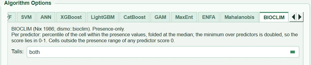
Family and implementation. Presence-only envelope method (Nix 1986). Written with numpy (sdm_niche.py:44-90). For each predictor, the percentile p of the cell value among the presence values is computed with the mid-rank rule; if p > 0.5, 1-p is taken (folded at the median); the minimum over predictors is taken and multiplied by two. The result lies between 0 and 1: 1 means at the median of all predictors, 0 means outside the presence range of at least one predictor. The score is not rescaled. Categorical variables are left out; at least 2 presences are needed.
| Name in the UI | What it does | Default | Range / options | Code |
|---|---|---|---|---|
Tails: |
Which tail lowers the score | both |
both, low, high |
tabs/tab_models.py:900-907; sdm_niche.py:79-88 |
5.19.1 Tails
- What it does.
bothis classical BIOCLIM: both tails lower the score.lowcounts only the lower tail (above the median 1, and above the presence range also 1);highcounts only the upper tail. It has the same meaning as dismopredict(…, tails=). - When and how to set it. If all variables are thought to be limiting in one direction only (e.g. minimum temperatures only),
loworhighis chosen. The choice is applied to all predictors. - Effect on results.
loworhighgives a wider suitable area thanboth. - Caution. The UI has no separate tail choice per predictor.
Comparison with R. Same definition as dismo bioclim. The percentile is computed with the mid-rank; because the way dismo handles ties could not be verified, values may differ at the 1/n level (sdm_niche.py:16-18).
5.20 Domain: Gower distance

Family and implementation. Presence-only similarity method (Carpenter et al. 1993). The Gower distance between a cell and each presence is the mean over predictors of \lvert x_j-z_j\rvert/\text{range}_j, where \text{range}_j is the range of the presence values. Suitability is \max(0,\,1-\min_z G) (sdm_niche.py:95-127). A predictor with zero range contributes 0 if equal and 1 otherwise. Categorical variables are left out; at least 2 presences are needed; duplicate presence rows are counted once.
It has no settings; the page contains only a description note (tabs/tab_models.py:917-925).
Caution: Domain looks at the single nearest presence. A single erroneous or extreme record creates high suitability around it; record cleaning (Chapter 2) is especially important for this method. Computation time increases linearly with the number of presences; memory is limited by processing cells in blocks.
Comparison with R. Same definition as dismo domain and flexsdm fit_dom; there is no comparison test in HABITUS.
5.21 GLMNET: elastic-net logistic regression
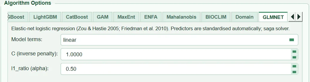
Family and implementation. Elastic-net logistic regression combining L1 and L2 penalties (Zou and Hastie 2005; Friedman et al. 2010). scikit-learn LogisticRegression, saga solver, at most 5000 iterations; terms are generated and standardised as in GLM (sdm_core.py:3446-3461, 3493-3505). Presence–pseudo-absence.
| Name in the UI | What it does | Default | Range / options | Code |
|---|---|---|---|---|
Model terms: |
Term structure | linear |
linear, quadratic, interactions |
tabs/tab_models.py:929-934 |
C (inverse penalty): |
Inverse penalty strength | 1.0000 | 0.0001 – 10 000 | tabs/tab_models.py:935-939 |
l1_ratio (alpha): |
L1 / L2 mixture | 0.50 | 0.0 – 1.0 (step 0.1) | tabs/tab_models.py:940-945 |
5.21.1 C (inverse penalty)
- What it does. If the scikit-learn objective function is divided by n to bring it into glmnet form, \lambda \approx 1/(C\,n); n is the number of training rows.
- When and how to set it. In the example run a training fold has about 860 rows; C = 1 means \lambda \approx 0.0012 and is a light penalty. For a real choice, the tuning tab tries C = 0.01/0.1/1/10.
- Effect on results. As C decreases, the coefficients shrink; if l1_ratio > 0, some predictors drop out entirely.
- Caution. R glmnet usually selects λ with
cv.glmnet; HABITUS uses a single fixed C.
5.21.2 l1_ratio (alpha)
- What it does. It is glmnet's
alpha: 0 is ridge (L2 only), 1 is lasso (L1 only; drops variables), in between is elastic net. - When and how to set it. If there are strongly correlated predictors, a value around 0.5 softens the lasso's tendency to pick one of the correlated variables at random.
- Effect on results. As it approaches 1, the model becomes sparser and easier to interpret.
- Caution.
sagamay converge slowly; with very small C and many terms a convergence warning may appear.
5.21.3 Model terms
- What it does. The same as GLM (§5.6.1); here the default is
linear(like the glmnet of the sdm package). - When and how to set it. Because the penalty slows overfitting,
quadraticorinteractionscan be tried with more confidence than in GLM (tooltip). - Effect on results. As terms increase, flexibility increases; the penalty can set superfluous terms to zero.
- Caution. The tuning tab does not change the term structure; the value here stays fixed.
5.22 CART: classification tree
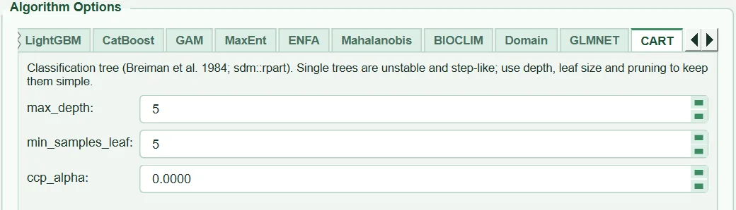
Family and implementation. A single classification tree (Breiman et al. 1984). scikit-learn DecisionTreeClassifier; suitability is the proportion of presences in the leaf into which the cell falls (sdm_core.py:3506-3515). Presence–pseudo-absence.
| Name in the UI | What it does | Default | Range / options | Code |
|---|---|---|---|---|
max_depth: |
Maximum depth | 5 | 0 (no limit) – 30 |
tabs/tab_models.py:957-960; sdm_core.py:3509-3511 |
min_samples_leaf: |
Minimum rows in a leaf | 5 | 1 – 500 | tabs/tab_models.py:961-963 |
ccp_alpha: |
Cost-complexity pruning | 0.0000 | 0.0 – 0.5 | tabs/tab_models.py:964-967 |
5.22.1 max_depth and min_samples_leaf
- What it does. The maximum depth of the tree (0 = unlimited) and the leaf size.
- When and how to set it. For explanatory use, a depth of 3–5 gives a readable tree. Because leaf proportions are the probabilities, very small leaves produce a 0/1 surface (tooltip).
- Effect on results. As depth increases, the map is divided into more stepped regions and training fit increases.
- Caution. A single tree is unstable: when the data change slightly, the structure of the tree can change considerably.
5.22.2 ccp_alpha
- What it does. Prunes the tree according to the complexity cost of each added leaf; it is the counterpart of rpart's
cpparameter, but its scale is not the same. - When and how to set it. The tuning tab tries 0/0.002/0.01.
- Effect on results. As it grows, the tree becomes smaller.
- Caution. rpart prunes with
cp= 0.01 by default; HABITUS's default is 0 (no pruning), and the limiting is done by depth and leaf size.
5.23 ESM: ensemble of small models
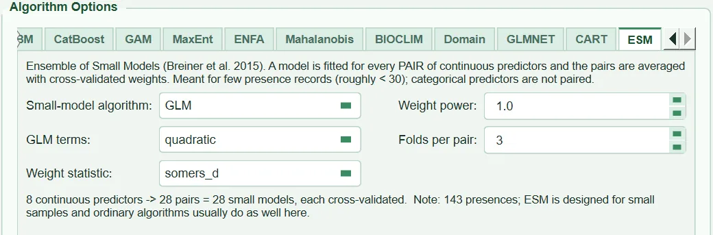
Family and implementation. The method recommended for species with very few records (Lomba et al. 2010; Breiner et al. 2015). For each pair of continuous predictors a small bivariate model is fitted; the pairs are weighted by their own cross-validation performance and averaged (sdm_core.py:4370-4455, sdm_niche.py:130-265). With p predictors there are p(p-1)/2 pairs; 28 with 8 predictors. Categorical variables do not enter the pairs. If there are more than 100 pairs, a warning is given (sdm_niche.py:39).
| Name in the UI | What it does | Default | Range / options | Code |
|---|---|---|---|---|
Small-model algorithm: |
Algorithm of the small models | GLM |
GLM, RF, MAXENT |
tabs/tab_models.py:979-983; sdm_core.py:4380-4385, 4407-4414 |
GLM terms: |
Terms of the GLM small models | quadratic |
quadratic, linear |
tabs/tab_models.py:1004-1005; sdm_core.py:4409 |
Weight statistic: |
Criterion for the pair weight | somers_d |
somers_d, auc, boyce |
tabs/tab_models.py:984-991; sdm_niche.py:142-157 |
Weight power: |
Exponent of the weight | 1.0 | 0.0 – 10.0 | tabs/tab_models.py:992-996 |
Folds per pair: |
Number of folds that score each pair | 3 | 2 – 10 | tabs/tab_models.py:997-1003; sdm_core.py:4296-4368 |
The information line at the bottom of the page computes the number of pairs from the selected predictors; with 50 or more presences it reminds the user that ESM is designed for small samples (tabs/tab_models.py:1022-1044).
5.23.1 Small-model algorithm and GLM terms
- What it does. The model of each pair. GLM is fitted with the same settings as the main GLM (C = 1) and the terms selected here; RF with 200 trees and leaf size 2 (cannot be changed in the UI); MaxEnt with the settings in the MaxEnt tab and the relevant two columns of the MaxEnt background (
sdm_core.py:4407-4445). - When and how to set it. A linear + quadratic GLM is the usual choice (Breiner et al. 2015). RF is slower, MaxEnt much slower. The default of flexsdm's
esm_glmis the linear term only; for comparison with it,linearis chosen. - Effect on results. Quadratic terms allow an optimum response in each pair.
- Caution.
Balance classesis applied to the small models only with the GLM and RF bases; with the MaxEnt base it is ignored and "not supported (ignored)" is written to the record (sdm_core.py:4402-4406).
5.23.2 Weight statistic and Weight power
- What it does. The weight of each pair is the criterion computed from the pair's out-of-fold predictions raised to the power
power.somers_d= \max(2(\text{AUC}-0.5),\,0);auc= raw AUC;boyce= \max(\text{Boyce},\,0). A pair no better than chance gets weight 0 withsomers_dandboyce. - When and how to set it. Breiner et al. (2015) use Somers' D.
aucweights are almost equal; to make them discriminating, the exponent should be chosen greater than 1. An exponent of 0 means equal weights. - Effect on results. As the exponent grows, the ensemble concentrates on the best few pairs.
- Caution. If no pair is better than chance, equal weights are used and the warning "No small model beat chance in cross-validation; the ensemble uses equal weights." is given (
sdm_niche.py:260-263).
5.23.3 Folds per pair
- What it does. The number of inner folds in which the pairs are scored. The folds apply the main cross-validation design (spatial block, environmental, band, checkerboard) to the rows on which ESM is trained; if the design cannot be applied or the design is
random/jackknife, random stratified folds are used (sdm_core.py:4296-4368). The number of folds cannot exceed the number of presences. - When and how to set it. With very few presences (10–20) 2–3 folds; with more presences 4–5.
- Effect on results. As folds increase, the weights become more stable and run time longer.
- Caution. When the design cannot be applied, the warning "ESM: the … design could not be applied to the folds that weight the small models (…); random stratified folds were used for them." is given once.
Comparison with R. ecospat ecospat.ESM.Modeling implements the same idea with biomod2 models. HABITUS's implementation is its own; there is no numerical comparison test against ecospat.
5.24 Outputs and what passes to the next step
- Saved settings: all values on this page (including those of unticked algorithms) go to the
habitus_run_config.json→settings.models.algorithm_optionsfield; the settings actually passed to MaxEnt (maxent_settings_used: elapid arguments, seed, number of presences added to the background, solver) are written separately. If ESM was run, the number of pairs, the weights and the ten best pairs are written to theesmfield (sdm_core.py:4457-4478). How class balancing was applied to each algorithm is in theclass_weight_appliedfield. - Models: each algorithm × PA set × fold and the full model; scores in the
Evaluation Resultssub-tab of ③, response curves, importance plots and ROC curves in ④ Evaluation. - Maps: current suitability per algorithm and the ensemble map (
Current Distribution Map), projection with the same models in ⑤ Future Scenarios.
5.25 Expert questions
Q1. Which of the eighteen algorithms should I choose; why are only GLM and RF the default?
Answer: At start-up the program ticks only GLM and RF (tabs/tab_models.py:129-132): one an interpretable parametric regression, the other a flexible tree ensemble; neither requires an additional package and both are fast. The code contains no definitive rule for the choice. A typical study runs several methods from different families (GLM or GAM, RF or BRT, MaxEnt) and combines them in an ensemble map. With very few records (below about 30), ESM, GLMNET or MaxEnt with linear/quadratic features; where there are only presence records and working with pseudo-absences is not wanted, MaxEnt, ENFA, Mahalanobis, BIOCLIM and Domain are considered. Valavi et al. (2022) examine comparative performance on presence-only data across many species; their results cannot be transferred directly to HABITUS's implementations, but they can still be consulted for the general behaviour of method families.
Q2. Where do the default values come from?
Answer: From three sources. (1) Library defaults: RF (500 trees, sqrt, leaf 1; the same as randomForest), SVM, ANN's alpha, GAM (20 splines, lam 0.6; pygam), XGBoost's penalties. (2) Publications: BRT learning rate and bagging fraction from Elith et al. (2008) (sdm_core.py:3530-3548), MaxEnt number of hinges and β = 1 from maxnet, ESM from Breiner et al. (2015). (3) HABITUS's own paired cross-validation comparisons: GBM's stumps and BRT's depth of 2 (code comments sdm_core.py:3517-3522, 3532-3537), GLM's C = 1 penalty (tooltip, tabs/tab_models.py:741-745). The details of these comparisons are in the internal notes referred to in the code comments; they are not the subject of this book. In a publication, settings should be reported not as "HABITUS defaults" but with the numbers in habitus_run_config.json.
Q3. Does HABITUS's MaxEnt give the same result as R maxnet?
Answer: The objective function is the same: per-feature L1 penalty, weights of presence 1 / background 100, last λ, addition of presences to the background (sdm_core.py:3776-3836, 4698-4707). tests/test_maxent_maxnet.py checks, on the data of Rutrough et al. (2019) at three settings, that the correlation with R maxnet 0.1.4 predictions exceeds 0.995 and that the mean absolute difference stays below 0.02. The remaining differences come from the solver (liblinear instead of glmnet's coordinate descent) and from the very small but non-zero penalty on the intercept. Feature generation belongs to elapid; the placement of hinge knots by elapid and maxnet agrees on this test dataset but has not been tested separately for every dataset. For an exact comparison with maxnet, Auto (maxnet default rule) should be ticked; HABITUS's default linear,hinge,product set is not the same as the maxnet rule.
Q4. Why is adding presences to the background important in MaxEnt?
Answer: This is the default behaviour of Maxent and maxnet; the environment where a presence occurs is also part of the available environment. If they are not added, the environment of presence cells is under-represented in the background distribution and the model's raw output and normalisation constant diverge from maxnet. HABITUS adds only presences whose predictor values are not already in the background (sdm_core.py:4702-4706); in the full model of the example run, 91 of the 143 presences were added.
Q5. Why are presence-only methods (MaxEnt, ENFA, Mahalanobis, BIOCLIM, Domain) evaluated with pseudo-absences?
Answer: HABITUS scores all algorithms in the same test fold with the same presence and pseudo-absence rows (sdm_core.py:5530-5540); in this way the scores are comparable across algorithms and the ensemble weights are consistent. In this case AUC is the power to "separate presence from pseudo-absence", not performance against true absence; the Boyce index, which relies on presences only, is a more suitable measure for presence-only data. If no presence remains in the test fold, one fifth of the training presences is moved to the test set (sdm_core.py:5455-5468); in that case the fold differs from the fold of the other algorithms. A user who wants to evaluate presence-only models separately should focus on the Boyce and OR_10p columns.
Q6. Should class balancing (Balance classes) be turned on; what does prevalence change?
Answer: The default is off. In the example run the pseudo-absence : presence ratio is 7.0 : 1 (pa_to_presence_ratio = 6.993). When balancing is turned on, the total weights of the two classes are equalised in the supported algorithms (§5.4.5). This changes the meaning of the predicted value: the output no longer reflects the pseudo-absence ratio, thresholds are re-derived; ranking measures (AUC) are mostly little affected (tooltip, tabs/tab_models.py:346-348). Because the number of pseudo-absences is arbitrary anyway, balancing is not required if absolute "probability" is not interpreted. What matters is that balancing is not applied at all in GAM, MaxEnt and the presence-only methods; balanced and unbalanced models can be mixed in one ensemble. A breakdown of how it was applied is in the class_weight_applied field.
Q7. Are the results reproducible; which sources add randomness?
Answer: Yes, with a single seed. All random learners are given the seed from ① Data (sdm_core.py:3474-3475); random_state is also passed to MaxEnt (sdm_core.py:4643), and permutation importance is computed with a generator derived from the seed (sdm_core.py:4847-4853). The settings that add randomness are RF's bootstrap, the subsampling of GBM/BRT/XGBoost/LightGBM, CatBoost's random_strength and bagging_temperature, ANN's initial weights, SVM's Platt folds and ESM's inner folds. Multithreaded libraries (RF, XGBoost, LightGBM n_jobs = -1) may give differences in the last digits on a different number of processors because of the floating-point summation order; this has not been tested in the code. Library versions are recorded in the habitus_run_config.json → environment field; the same versions are needed for the same result.
Q8. Why is GLM penalised; how do I compare my result with glm in R?
Answer: Quadratic and interaction terms inflate the coefficients with few records; HABITUS applies a light L2 penalty to the standardised terms (sdm_core.py:3481-3492). R glm() is unpenalised. For comparison, enter Regularisation C = 1e6; the term structure is built in R with y ~ x + I(x^2) (quadratic) or y ~ poly(x1, x2, degree = 2, raw = TRUE) (interactions). biomod2's GLM additionally performs stepwise selection by AIC; HABITUS has no stepwise selection, so the coefficients will not be exactly the same as biomod2's.
Q9. Why can GAM results differ from mgcv?
Answer: HABITUS fits pygam LogisticGAM with a fixed smoothing penalty (lam, default 0.6) and 20 B-spline bases per predictor (sdm_core.py:4500-4523). mgcv, in contrast, selects the penalty from the data (GCV/REML) and uses a different basis. On the same data mgcv may choose a smoother or a more wiggly curve. To bring them closer, lam can be searched in the tuning tab; but the two models will still not be identical. GAM has no interaction terms and no class balancing.
Q10. Does BRT select the number of trees itself like dismo gbm.step?
Answer: No. n_estimators is fixed (BRT 1000, GBM 200) and early stopping is not used (sdm_core.py:3523-3548). dismo gbm.step stops the number of trees where the 10-fold cross-validation deviance is smallest. For a similar result in HABITUS, an n_estimators × learning_rate grid is searched in the GBM tuning tab and the selected value is written into BRT by hand. Also, whereas Elith et al. used tree.complexity = 5, HABITUS BRT's depth is 2.
Q11. Are the defaults of XGBoost, LightGBM and CatBoost suitable for SDM?
Answer: The defaults of these three (XGBoost depth 6 and 500 rounds; LightGBM 31 leaves, unlimited depth and 500 rounds; CatBoost depth 4 and 300 rounds) are much more complex models than GBM and BRT (sdm_core.py:3586-3647). The comparison table in the help tab notes at least 100 records and a tendency to overfit for them. With data of fewer than a few hundred presences it is recommended to reduce depth to 2–3 and the number of leaves to 7–15 and to check the result with the training–test AUC difference (dAUC). Note that the subsample setting has no effect in LightGBM (§5.13.3).
Q12. When I add a categorical predictor (e.g. land cover), does every algorithm use it in the same way?
Answer: No (§5.4.3). Regression and kernel methods use one 0/1 column per class, GAM a factor term, MaxEnt a categorical feature; tree methods handle the integer code with numeric splits; envelope and distance methods leave the variable out and write a note to the log (sdm_core.py:4010-4036). So some of the models in an ensemble may not see the categorical variable at all. A class not seen in training (present only in the projection area) is treated as "no class effect" in regression methods, GAM and MaxEnt, and in trees it is evaluated in the branch into which its numeric code falls.
Q13. Why are ENFA and Mahalanobis scores rescaled to the range 0–1; is the map comparable?
Answer: The raw score \exp(-D^2/2) approaches zero quickly with many predictors. HABITUS stores the score range of the training rows during fitting and uses the same range in every prediction (sdm_core.py:3719-3743). Therefore a cell gets the same value in the test fold and in the projection, and the threshold has the same meaning in both settings. Even so, the scale of the score is specific to the algorithm; 0.6 from ENFA and 0.6 from GLM are not the same probability. Ensemble weights and binary thresholds are therefore determined separately per algorithm (Chapter 6).
Q14. How should I report the tuned parameters in a publication?
Answer: algorithm_options (the values entered), maxent_settings_used (what was actually passed to MaxEnt, and the solver), class_weight, clamp, random_seed and environment (library versions) in habitus_run_config.json should be reported together. If the tuning tab was used, the grid, the selection rule and the selected point should also be stated; that the score may be optimistic when tuning and evaluation are done on the same folds is discussed in Chapter 6. The ODMAP report (Chapter 11) carries most of this information automatically.
5.26 Common mistakes and pitfalls
- Package not installed: the box is grey with
[not installed]appended. Example tooltip: "Not installed — pip install elapid". After installation the program must be restarted. - Running without selecting any algorithm: "Select at least one algorithm."
- Writing the ANN layers incorrectly (e.g.
100;50,100 50,0): "ANN hidden layers: … is not a list of positive whole numbers separated by commas (e.g. 100, 50)." - Writing
autoor%50in RFmax_features: "RF max_features: … is not sqrt, log2, a whole number of variables or a fraction between 0 and 1." The fraction should be written as 0.5. - GAM
n_splines≤ 3: the UI lower limit is 4; if given by script, "GAM n_splines must exceed the spline order (3)." - Misspelling a MaxEnt feature name (e.g.
hinges,quad): elapid rejects the setting and MaxEnt fails with the message "MaxEnt could not be fitted…" or "MaxEnt could not be configured with the settings you chose…". Valid names:linear,quadratic,hinge,product,threshold. - Changing the text box in MaxEnt while
Autois ticked: the box is disabled and ignored. - Changing
N threshold featureswithout selecting thethresholdclass: the value is not used. - Giving categorical variables to presence-only methods: the variable is left out, not silently, but with the message "NOTE: … is an envelope/distance model for continuous predictors…" in the log; if there are only categorical variables, the error "… needs at least one continuous predictor (only categorical ones were given)." is given.
- Running ESM with many predictors: 15 predictors means 105 pairs and 105 separate cross-validated models; the information line says "WARNING: more than 100 pairs…".
- Using ESM for a species with many records: with 50 or more presences the information line reminds the user that ESM is designed for small samples; the usual algorithms are generally as good.
LinAlgErrorin Mahalanobis: increase ε or keep Ledoit–Wolf on; strongly correlated predictors are removed in ② Variables.- Assuming that
Balance classesaffects every algorithm: it has no effect in GAM, MaxEnt, ENFA, Mahalanobis, BIOCLIM and Domain. - Adjusting LightGBM
subsample: because row subsampling is not active in HABITUS, the value does not change the result. - Using the default deep boosting models with few records: in XGBoost/LightGBM, training AUC approaches 1 while test AUC falls; the dAUC column should be monitored.
5.27 References
Anderson, C.B., 2023. elapid: Species distribution modeling tools for Python. Journal of Open Source Software 8, 4930. https://doi.org/10.21105/joss.04930
Breiman, L., 2001. Random forests. Machine Learning 45, 5–32. https://doi.org/10.1023/A:1010933404324
Breiman, L., Friedman, J.H., Olshen, R.A., Stone, C.J., 1984. Classification and Regression Trees. Wadsworth, Belmont (new edition: Routledge, 2017). https://doi.org/10.1201/9781315139470
Breiner, F.T., Guisan, A., Bergamini, A., Nobis, M.P., 2015. Overcoming limitations of modelling rare species by using ensembles of small models. Methods in Ecology and Evolution 6, 1210–1218. https://doi.org/10.1111/2041-210X.12403
Carpenter, G., Gillison, A.N., Winter, J., 1993. DOMAIN: a flexible modelling procedure for mapping potential distributions of plants and animals. Biodiversity and Conservation 2, 667–680. https://doi.org/10.1007/BF00051966
Chen, T., Guestrin, C., 2016. XGBoost: A scalable tree boosting system. Proceedings of the 22nd ACM SIGKDD International Conference on Knowledge Discovery and Data Mining, 785–794. https://doi.org/10.1145/2939672.2939785
Elith, J., Leathwick, J.R., Hastie, T., 2008. A working guide to boosted regression trees. Journal of Animal Ecology 77, 802–813. https://doi.org/10.1111/j.1365-2656.2008.01390.x
Farber, O., Kadmon, R., 2003. Assessment of alternative approaches for bioclimatic modeling with special emphasis on the Mahalanobis distance. Ecological Modelling 160, 115–130. https://doi.org/10.1016/S0304-3800(02)00327-7
Friedman, J., Hastie, T., Tibshirani, R., 2010. Regularization paths for generalized linear models via coordinate descent. Journal of Statistical Software 33(1), 1–22. https://doi.org/10.18637/jss.v033.i01
Hastie, T., Tibshirani, R., 1986. Generalized additive models. Statistical Science 1, 297–310. https://doi.org/10.1214/ss/1177013604
Hirzel, A.H., Hausser, J., Chessel, D., Perrin, N., 2002. Ecological-niche factor analysis: how to compute habitat-suitability maps without absence data? Ecology 83, 2027–2036. https://doi.org/10.1890/0012-9658(2002)083[2027:ENFAHT]2.0.CO;2
Ledoit, O., Wolf, M., 2004. A well-conditioned estimator for large-dimensional covariance matrices. Journal of Multivariate Analysis 88, 365–411. https://doi.org/10.1016/S0047-259X(03)00096-4
Lomba, A., Pellissier, L., Randin, C., Vicente, J., Moreira, F., Honrado, J., Guisan, A., 2010. Overcoming the rare species modelling paradox: a novel hierarchical framework applied to an Iberian endemic plant. Biological Conservation 143, 2647–2657. https://doi.org/10.1016/j.biocon.2010.07.007
Merow, C., Smith, M.J., Silander, J.A., 2013. A practical guide to MaxEnt for modeling species' distributions: what it does, and why inputs and settings matter. Ecography 36, 1058–1069. https://doi.org/10.1111/j.1600-0587.2013.07872.x
Muscarella, R., Galante, P.J., Soley-Guardia, M., Boria, R.A., Kass, J.M., Uriarte, M., Anderson, R.P., 2014. ENMeval: An R package for conducting spatially independent evaluations and estimating optimal model complexity for Maxent ecological niche models. Methods in Ecology and Evolution 5, 1198–1205. https://doi.org/10.1111/2041-210X.12261
Nix, H.A., 1986. A biogeographic analysis of Australian elapid snakes. In: Longmore, R. (Ed.), Atlas of Elapid Snakes of Australia. Australian Flora and Fauna Series 7. Australian Government Publishing Service, Canberra, 4–15.
Oshiro, T.M., Perez, P.S., Baranauskas, J.A., 2012. How many trees in a random forest? In: Perner, P. (Ed.), Machine Learning and Data Mining in Pattern Recognition. Lecture Notes in Computer Science 7376. Springer, Berlin, 154–168. https://doi.org/10.1007/978-3-642-31537-4_13
Phillips, S.J., Anderson, R.P., Schapire, R.E., 2006. Maximum entropy modeling of species geographic distributions. Ecological Modelling 190, 231–259. https://doi.org/10.1016/j.ecolmodel.2005.03.026
Phillips, S.J., Anderson, R.P., Dudík, M., Schapire, R.E., Blair, M.E., 2017. Opening the black box: an open-source release of Maxent. Ecography 40, 887–893. https://doi.org/10.1111/ecog.03049
Rutrough, A., Widick, I.V., Bean, W.T., 2019. Reconstruction of the historical range alters niche estimates in an endangered rodent. Ecography 42, 1742–1751. https://doi.org/10.1111/ecog.04238
Valavi, R., Elith, J., Lahoz-Monfort, J.J., Guillera-Arroita, G., 2021. Modelling species presence-only data with random forests. Ecography 44, 1731–1742. https://doi.org/10.1111/ecog.05615
Valavi, R., Guillera-Arroita, G., Lahoz-Monfort, J.J., Elith, J., 2022. Predictive performance of presence-only species distribution models: a benchmark study with reproducible code. Ecological Monographs 92, e01486. https://doi.org/10.1002/ecm.1486
Velazco, S.J.E., Rose, M.B., de Andrade, A.F.A., Minoli, I., Franklin, J., 2022. flexsdm: An R package for supporting a comprehensive and flexible species distribution modelling workflow. Methods in Ecology and Evolution 13, 1661–1669. https://doi.org/10.1111/2041-210X.13874
Zou, H., Hastie, T., 2005. Regularization and variable selection via the elastic net. Journal of the Royal Statistical Society Series B 67, 301–320. https://doi.org/10.1111/j.1467-9868.2005.00503.x